Compare Inversion Calls Across Treatments

What would be interesting to see is the inversion-calling performance in linked reads across inversion sizes and depths. Since we already created the assessment tables from the individual size-class data exploration, we can read those in without having to reprocess those data.

library(ggplot2)
library(dplyr)
library(tidyr)
library(ggh4x)
options(warn = -1)

Read in the LEVIATHAN linked-read variant assessments. Remove the inversion and id columns. We will add the leviathan candidates as their own technology and do the same with the pooled data.

.lev <- read.csv("assess_sv_leviathan/visor/linkedread.sv.assessment", header = T) %>%
    select(-inversion, -id, -candidate)
.lev$technology[.lev$sample == 11] <- "linkedread (pooled)"
.lev$zygosity[.lev$sample == 11] <- "homozygous"

# rm pooled from the candidates
.lev_cand <- select(.lev, -assessment) %>% rename("assessment" = assess_cand) %>% filter(sample < 11)

# rename the false negative (filtered) to "true positive" to posit an ideal world where candidates were detected
.lev_cand$assessment[grepl("filtered", .lev_cand$assessment)] <- "true positive"
.lev_cand$assessment[grepl("undetected", .lev_cand$assessment)] <- "false negative"
.lev_cand$technology <- "linkedread (candidates)"

leviathan <- rbind(select(.lev, -assess_cand), .lev_cand)

table(leviathan$technology)
table(leviathan$assessment)
head(leviathan)


             linkedread linkedread (candidates)     linkedread (pooled) 
                   2400                    2400                     240


false negative  true negative  true positive 
          1236           1300           2504

naibr <- read.csv("assess_sv_naibr/visor/linkedread.sv.assessment", header = T) %>%
    select(-inversion, -id)
table(naibr$assessment)
head(naibr)


false negative  true negative  true positive 
          1323            650            667

For the short reads, we can rename the values in the technology column as shortread

delly <- read.csv("assess_sv_delly/linkedread.sv.assessment", header = T)
delly$technology <- "shortread"
delly <- select(delly, -inversion, -id)
table(delly$assessment)
head(delly)


false negative  true negative  true positive 
           407            650           1343

Read in the long-read variant assessment. Rename the columns because I clearly wasn’t consistent doing this over and over again.

longread <- read.csv("longread_workflow/longread.sv.assessment", header = T)
longread <- rename(longread, "simulated" = present, "technology" = platform)
longread$method <- "sniffles"
longread$sample <- as.integer(gsub("sample_", "", longread$sample))
table(longread$assessment)
head(longread)


false negative  true negative  true positive 
          1194           1950           4056

assess <- rbind(leviathan, naibr, delly, longread)
head(assess)

Let’s also make some of the columns factors.

#assess$depth <- as.factor(assess$depth)
assess$size <- factor(assess$size, ordered = T, levels = c("small","medium","large","xl"))
assess$technology <- factor(assess$technology, ordered = T, levels = c("linkedread", "linkedread (pooled)", "linkedread (candidates)", "shortread", "ontshort", "ontlong", "pacbio"))
assess$zygosity <- as.factor(assess$zygosity)
assess$assessment <- as.factor(assess$assessment)
assess$method <- as.factor(assess$method)

head(assess, 10)

Sample-level Calling¶

Prepare the Data¶

It would probably make sense to collapse these data somewhat to show a representation of true positives vs false negatives (as a ratio) across depths (x axis) and faceted for hom/het. We will also remove inversions that weren’t simulated for a sample b/c we aren’t interested in true negatives (since there were no false positives). Let’s also remove naibr (for now).

.assess <- as.vector(outer(c("true", "false"), c("positive", "negative"), paste))
samples <- assess[assess$method != "naibr",] %>%
    group_by(size, depth, zygosity, assessment, technology) %>%
    summarize(count = n()) %>% ungroup() %>%
    complete(size, depth, zygosity, technology, assessment = .assess[c(-2)], fill = list(count = 0))

head(samples)

`summarise()` has grouped output by 'size', 'depth', 'zygosity', 'assessment'.
You can override using the `.groups` argument.

Pop out the true negatives for a moment so we can get the proportion of TP vs FN

true_negs <- samples[samples$assessment == "true negative",]
true_negs$proportion <- 0
head(true_negs)

One last thing we’ll need to do is convert counts to proportions.

samples <- filter(samples, assessment != "true negative") %>%
    group_by(size, depth, zygosity, technology) %>%
    mutate(proportion = round(count/sum(count),2)) %>% ungroup()

# add the true negatives back in
samples <- rbind(samples, true_negs)
head(samples)

Let’s also set a color palette for the technology comparisons using the Arches theme and the Redwoods theme for the depths.

tech_colors <- c(
    "ontshort" = "#9b6981",
    "ontlong" = "#682c37",
    "pacbio" = "#f6955e" ,
    "linkedread" = "#a8cdec",
    "linkedread (pooled)" = "#a8cdec",
    "linkedread (candidates)" = "#a8cdec",
    "shortread" = "#7285c3ff"
)

size_colors <- c(
    "#c0c6cf",
    "#a2aab5",
    "#6e7684",
    "#54546c"
)

depth_colors <- c(
    "#c0c6cf",
    "#a2aab5",
    "#6e7684",
    "#54546c",
    "#30303dff"
)

zygosity_colors <- c(
    "#85a98eff",
    "#7fa9b4ff"
)

technology_lines <- c(
    "linkedread" = "solid",
    "linkedread (pooled)" = "dotdash",
    "linkedread (candidates)" = "dashed",
    "shortread" = "solid", 
    "ontshort" = "solid",
    "ontlong" = "solid",
    "pacbio" = "solid"
)

technology_shapes <- c(
    "linkedread" = 17,
    "linkedread (pooled)" = 17,
    "linkedread (candidates)" = 17,
    "shortread" = 25, 
    "ontshort" = 19,
    "ontlong" = 15,
    "pacbio" = 18
)

technology_shapes2 <- c(
    "linkedread" = 17,
    "linkedread (pooled)" = 25,
    "linkedread (candidates)" = 18,
    "shortread" = 19, 
    "ontshort" = 19,
    "ontlong" = 19,
    "pacbio" = 19
)

Visualization¶

We are now interested in seeing how these performed. There are several dimensions to consider here:

depth
inversion size
zygotic state
sequencing technology

Detection between technologies across inversion classes¶

We’ll approach this a few different ways to try to reveal meaningful information. First let’s compare how each of the technologies did within a given inversion size class.

options(repr.plot.width = 12, repr.plot.height = 12)
.strip <- strip_themed(background_x = elem_list_rect(fill = zygosity_colors), background_y = elem_list_rect(fill = size_colors))

filter(samples, assessment == "true positive") %>%
ggplot(aes(x = depth, y = proportion, color = technology, fill = technology, group = technology, shape = technology)) +
    geom_line(aes(linetype = technology)) +
    geom_point(size = 4) +
    scale_linetype_manual(values = technology_lines) +
    scale_color_manual(values = tech_colors) +
    scale_fill_manual(values = tech_colors) +
    scale_shape_manual(values = technology_shapes) +
    theme_light() +
    labs(
        title = "Inversion Detection by Zygotic State and Variant Size",
        subtitle = "Linked-reads us LEVIATHAN detections",
        color = "Technology", shape = "Technology", fill = "Technology", linetype = "Technology") +
    ylab("Proportion of Inversions Correctly Detected") +
    xlab("Sequencing Depth") +
    theme(panel.grid.minor.y = element_blank(), panel.grid.major.x = element_blank()) +
    facet_grid2(cols = vars(zygosity), rows = vars(size), strip = .strip)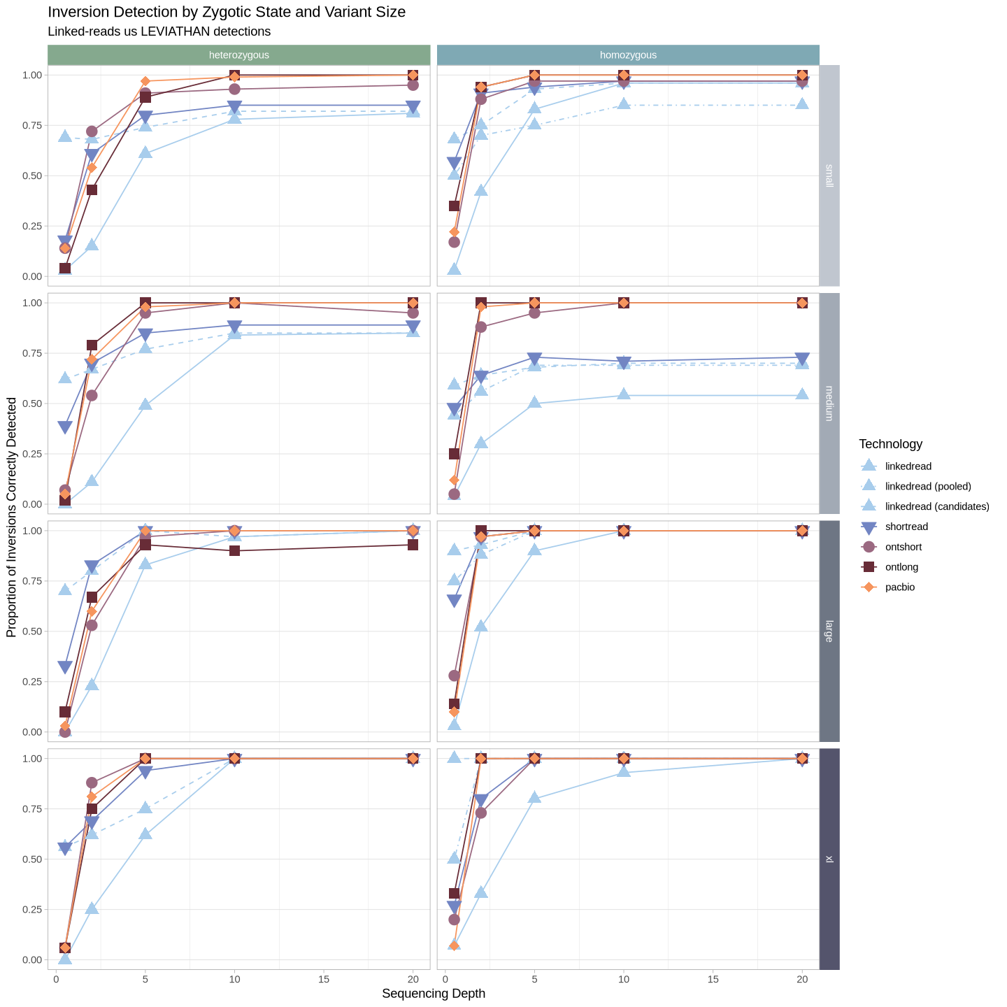

Can also flip it horizontally

options(repr.plot.width = 18, repr.plot.height = 8)
.strip <- strip_themed(background_y = elem_list_rect(fill = zygosity_colors), background_x = elem_list_rect(fill = size_colors))

filter(samples, assessment == "true positive") %>%
ggplot(aes(x = depth, y = proportion, color = technology, fill = technology, group = technology, shape = technology)) +
    geom_line(aes(linetype = technology)) +
    geom_point(size = 4) +
    scale_linetype_manual(values = technology_lines) +
    scale_color_manual(values = tech_colors) +
    scale_fill_manual(values = tech_colors) +
    scale_shape_manual(values = technology_shapes) +
    theme_light() +
    labs(
        title = "Inversion Detection by Zygotic State and Variant Size",
        subtitle = "Linked-reads us LEVIATHAN detections",
        color = "Technology", shape = "Technology", fill = "Technology", linetype = "Technology") +
    ylab("Proportion of Inversions Correctly Detected") +
    xlab("Sequencing Depth") +
    theme(panel.grid.minor.y = element_blank(), panel.grid.major.x = element_blank()) +
    facet_grid2(rows = vars(zygosity), cols = vars(size), strip = .strip)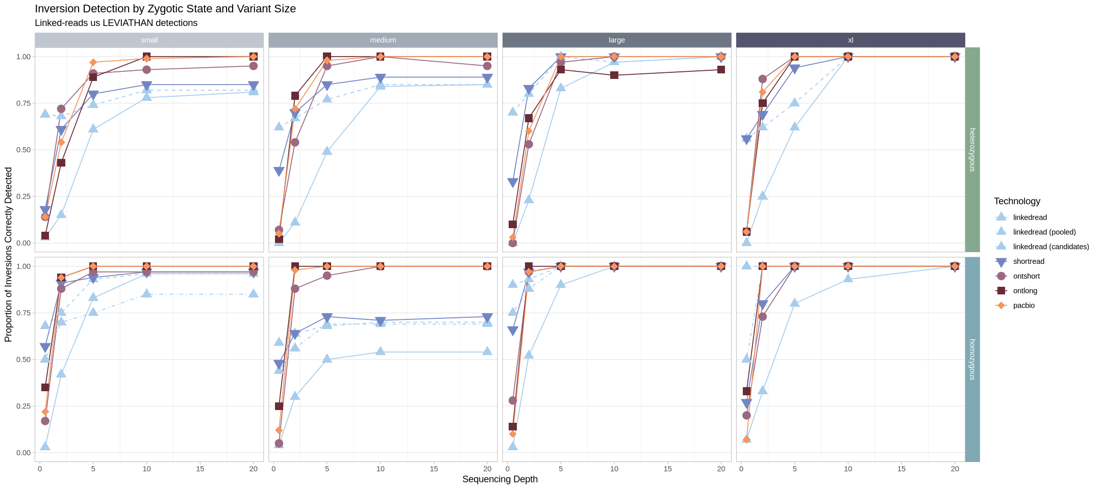

Detection between inversion class within technologies¶

This is effectively the same thing, but it’s a more 1:1 comparison across size classes within a given technology.

options(repr.plot.width = 8, repr.plot.height = 14)
.strip <- strip_themed(background_x = elem_list_rect(fill = zygosity_colors), background_y = elem_list_rect(fill = tech_colors[c(4,4,4,7,1,2,3)]))

filter(samples, assessment == "true positive") %>%
ggplot(aes(x = depth, y = proportion, color = size, group = size, shape = size)) +
    geom_line() +
    geom_point(size = 4) +
    scale_shape_manual(values = c(19,15,18,17)) +
    scale_color_manual(values = size_colors) +
    theme_light() +
    labs(title = "Inversion Detection as a Product of Variant Size", color = "Inversion Size", shape = "Inversion Size") +
    ylab("Proportion of Inversions Correctly Detected") +
    xlab("Sequencing Depth") +
    theme(panel.grid.minor.y = element_blank(), panel.grid.major.x = element_blank()) +
    facet_grid2(cols = vars(zygosity), rows = vars(technology), strip = .strip)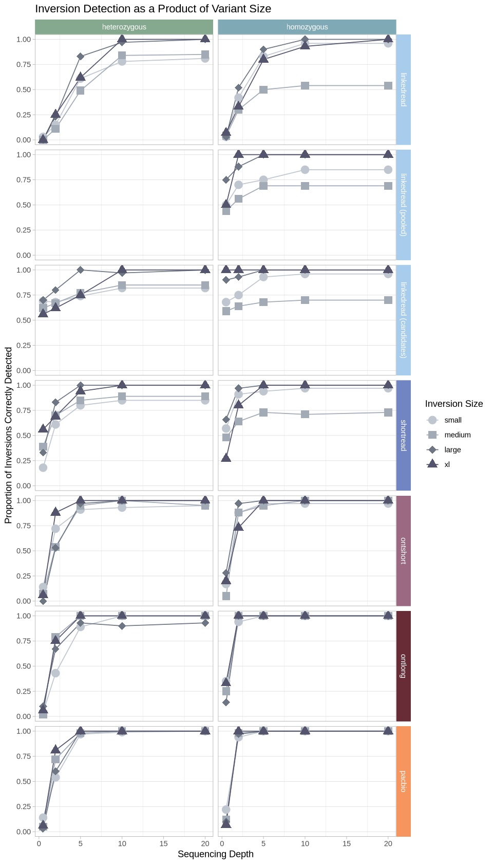

Can also show it horizontally

options(repr.plot.width = 18, repr.plot.height = 5)
.strip <- strip_themed(background_y = elem_list_rect(fill = zygosity_colors), background_x = elem_list_rect(fill = tech_colors[c(4,4,4,7,1,2,3)]))

filter(samples, assessment == "true positive") %>%
ggplot(aes(x = depth, y = proportion, color = size, group = size, shape = size)) +
    geom_line() +
    geom_point(size = 4) +
    scale_shape_manual(values = c(19,15,18,17)) +
    scale_color_manual(values = size_colors) +
    theme_light() +
    labs(title = "Inversion Detection as a Product of Variant Size", color = "Inversion Size", shape = "Inversion Size") +
    ylab("Proportion of Inversions Correctly Detected") +
    xlab("Sequencing Depth") +
    theme(panel.grid.minor.y = element_blank(), panel.grid.major.x = element_blank()) +
    facet_grid2(rows = vars(zygosity), cols = vars(technology), strip = .strip)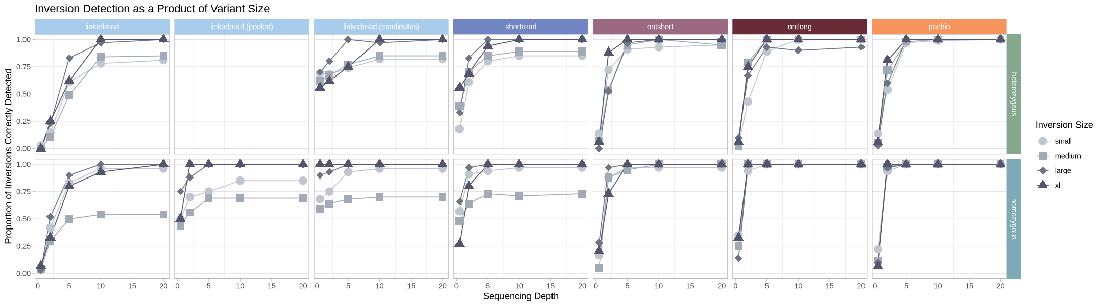

Holistic comparison of technologies¶

What does it look like when we compare the performance of hom/het within and across technologies for each inversion class?

options(repr.plot.width = 18, repr.plot.height = 4)
.strip <- strip_themed(background_x = elem_list_rect(fill = size_colors))

filter(samples, assessment == "true positive") %>%
ggplot(aes(x = depth, y = proportion, color = technology, group = paste(technology, zygosity), shape = zygosity)) +
    geom_line(aes(linetype = technology)) +
    geom_point(aes(shape = zygosity), size = 4) +
    theme_light() +
    scale_color_manual(values = tech_colors) +
    scale_linetype_manual(values = technology_lines) +
    scale_shape_manual(values = c("homozygous"= 19,"heterozygous" = 18)) +
    labs(title = "Inversion Detection as a Product of Zygotic State", linetype = "Technology", color = "Technology", shape = "Zygotic State") +
    ylab("Proportion of Inversions Correctly Detected") +
    xlab("Sequencing Depth") +
    theme(panel.grid.minor.y = element_blank(), panel.grid.major.x = element_blank()) +
    facet_grid2(cols = vars(size), strip = .strip)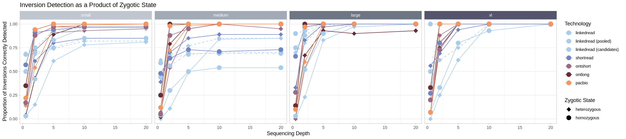

Let’s make it less busy by summing homozygous and heterozygous so it’s a total assessment agnostic of zygotic state.

samples_consolidated <- filter(samples, assessment != "true negative") %>%
    group_by(size, depth, technology, assessment) %>%
        summarise(count = sum(count)) %>%
        mutate(
            proportion = round(count/sum(count),2)
        ) %>% ungroup()
head(samples_consolidated)

`summarise()` has grouped output by 'size', 'depth', 'technology'. You can
override using the `.groups` argument.

filter(samples_consolidated, assessment == "true positive") %>%
ggplot(aes(x = depth, y = proportion, color = technology, group = technology)) +
    geom_line(aes(linetype = technology)) +
    geom_point(size = 4, aes(shape = technology)) +
    theme_light() +
    scale_color_manual(values = tech_colors) +
    scale_linetype_manual(values = technology_lines) +
    scale_shape_manual(values = technology_shapes2) +
    labs(title = "Inversion Detection across technologies", linetype = "Technology", color = "Technology", shape = "Technology") +
    ylab("Proportion of Inversions Correctly Detected") +
    xlab("Sequencing Depth") +
    theme(panel.grid.minor.y = element_blank(), panel.grid.major.x = element_blank()) +
    facet_grid2(cols = vars(size), strip = .strip)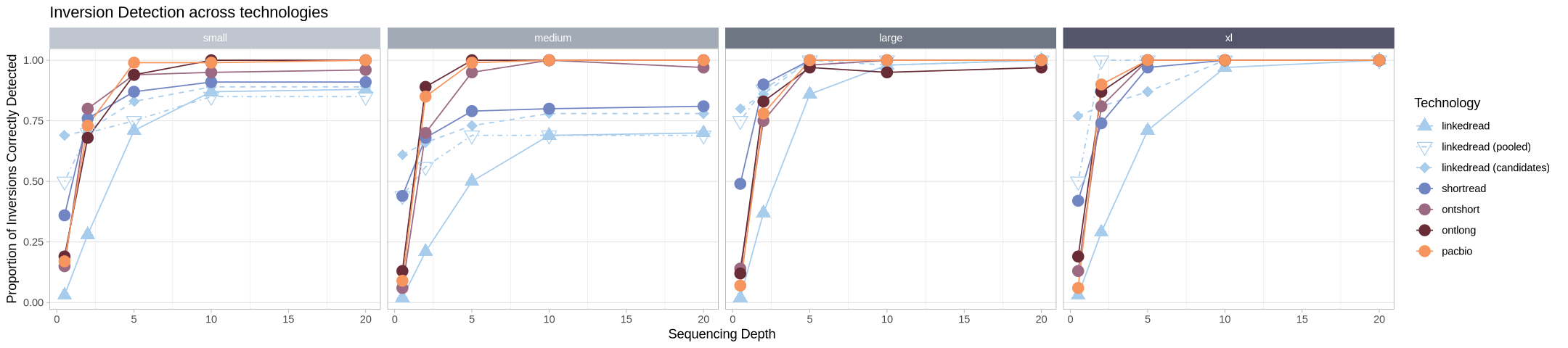

F-Score¶

Let’s look at the comparison of Precision vs Recall by using the F1 score. To start, we’ll need to read in all the false positives across the different methods.

# this function automates reading in everything all at once returns an empty table if there are no false positives
read.fp <- function(dir){
    val <- Reduce(
       rbind,
        Map(
            function(x){ read.table(x, header = T)},
            list.files(dir, pattern = "false_positives*", full.names = T)
        )
    )
    if (is.null(val)){
        return(
            data.frame(
                contig = character(),
                position_start = integer(),
                position_end = integer(),
                sample = integer(),
                depth = numeric(),
                size = character(),
                method = character()
            )
        )
    } else {
        return(val)
    }
}

false_positives <- Reduce(
    rbind,
    Map(
        read.fp,
        c("assess_sv_delly", "assess_sv_leviathan/visor", "longread_workflow")
    )
)

false_positives$assessment <- "false positive"
false_positives <- rename(false_positives, "technology" = method)
false_positives$technology <- gsub("delly", "shortread", false_positives$technology)
head(false_positives)

samples_consolidated_full <- group_by(samples, size, depth, technology, assessment) %>%
    summarise(count = sum(count)) %>% ungroup()

metrics <- group_by(false_positives, size, depth, assessment, technology) %>%
    summarize(count = n()) %>% ungroup() %>%
    rbind(samples_consolidated_full) %>%
    arrange(size, depth, technology, assessment) %>%
    filter(technology != "linkedread (candidates)") %>%
    complete(size, depth, technology, assessment = .assess, fill = list(count = 0)) %>%
    pivot_wider(names_from = assessment, values_from = count)
names(metrics) <- c("size", "depth", "technology", "FN", "FP", "TN", "TP")
head(metrics)

`summarise()` has grouped output by 'size', 'depth', 'technology'. You can
override using the `.groups` argument.
`summarise()` has grouped output by 'size', 'depth', 'assessment'. You can
override using the `.groups` argument.

metrics$precision <- metrics$TP / (metrics$TP + metrics$FP)
metrics$recall <- metrics$TP / (metrics$TP + metrics$FN)
metrics$F1 <- 2 * ((metrics$precision * metrics$recall) / (metrics$precision + metrics$recall))
metrics$depth <- metrics$depth
metrics$size <- factor(metrics$size, ordered = T, levels = c("small", "medium", "large", "xl"))
metrics$depth <- as.numeric(metrics$depth)
head(metrics)

options(warn = -1, repr.plot.width = 18, repr.plot.height = 5)
.strip <- strip_themed(background_x = elem_list_rect(fill = size_colors))
ggplot(metrics, aes(x = depth, y = F1, color = technology, shape = technology, group = technology)) +
    geom_line() +
    geom_point(size = 6) +
    theme_light() +
    scale_shape_manual(name = "Technology", values = technology_shapes2) +
    scale_color_manual(name = "Technology", values = tech_colors) +
    labs(title = "F-scores Across treatments") +
    facet_grid2(cols = vars(size), strip = .strip)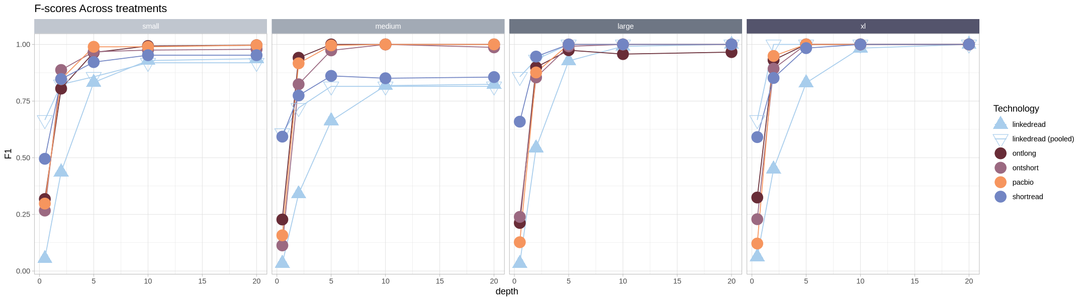

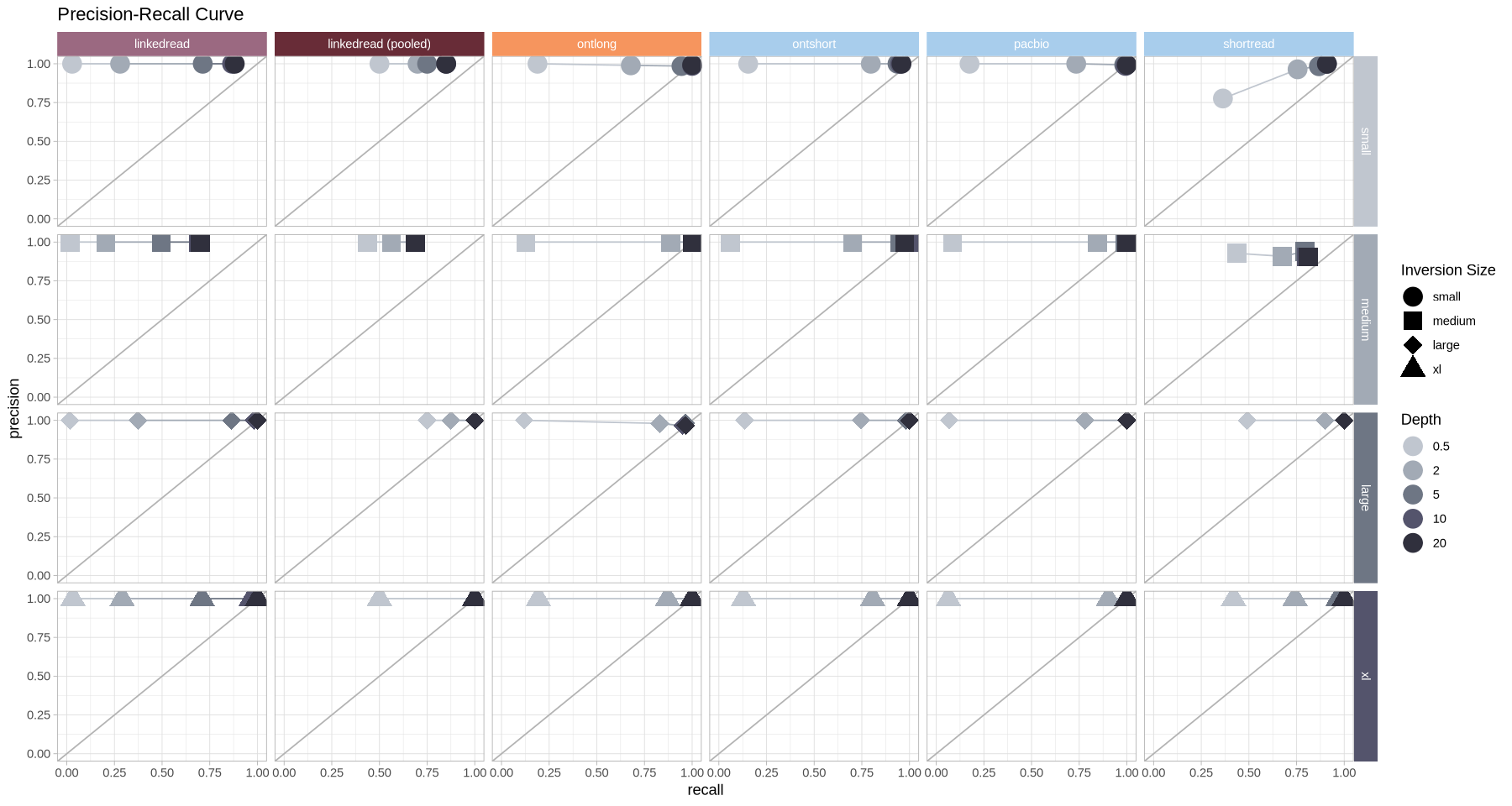
What about precision versus recall?

options(warn = -1, repr.plot.width = 15, repr.plot.height = 8)
.strip <- strip_themed(
    background_y = elem_list_rect(fill = size_colors),
    background_x = elem_list_rect(fill = tech_colors)
)

ggplot(metrics, aes(x = recall, y = precision, color = as.factor(depth), shape = size)) +
    geom_abline(intercept = 0, slope = 1, color = "grey70") +
    geom_line(aes(group = paste(technology, size))) +
    geom_point(size = 6) +
    theme_light() +
    scale_color_manual(name = "Depth", values = depth_colors) +
    scale_shape_manual(name = "Inversion Size", values = c(19,15,18,17)) +
    coord_cartesian(xlim = c(0,1), ylim = c(0,1)) +
    labs(title = "Precision-Recall Curve") +
    facet_grid2(cols = vars(technology), rows = vars(size), strip = .strip)