Long-Read (Sniffles) - Inversion Simulations

Here, we visualize the inversions that were identified across all size, depth, and platform treatments for long reads.

library(ggplot2)
library(dplyr)
library(tidyr)
library(ggpubr)
options(warn = -1, repr.plot.width = 19, repr.plot.height = 12)


Attaching package: 'dplyr'


The following objects are masked from 'package:stats':

    filter, lag


The following objects are masked from 'package:base':

    intersect, setdiff, setequal, union

Import Data¶

Identified Inversions¶

Read in the aggregate inversion discovery manifest

found_inversions <- read.table("longread.inversions.summary", header = T)
nrow(found_inversions)
head(found_inversions)

Simulated Inversions¶

Read in the groundtruth file. To avoid merging the breakpoints with the samples-inversions manifest each time, this process was done once with the code below and written to the file to be imported.

if(!file.exists("manifest.breakpoints")){
    # Get all the inversion breakpoints
    groundtruth <- read.table("../inversion_simulations.inventory", header = T)
    truthfile <- paste0("../simulated_variants/setup_inversions/small/inv.small.vcf")
    inversion_breakpoints <- read.table(truthfile, header = F)[,c(1,2,8)]
    inversion_breakpoints$V8 <- as.numeric(unlist(lapply(inversion_breakpoints$V8, function(X){gsub(".+END=", "", X)})))
    names(inversion_breakpoints) <- c("contig", "position_start", "position_end")
    inversion_breakpoints$size <- "small"
    inversion_breakpoints <- group_by(inversion_breakpoints, contig) %>% mutate(inversion = 1:n())

    for( i in c("medium", "large","xl") ){
        truthfile <- paste0("../simulated_variants/setup_inversions/", i, "/inv.", i,".vcf")
    
        .inversion_breakpoints <- read.table(truthfile, header = F)[,c(1,2,8)]
        .inversion_breakpoints$V8 <- as.numeric(unlist(lapply(.inversion_breakpoints$V8, function(X){gsub(".+END=", "", X)})))
        names(.inversion_breakpoints) <- c("contig", "position_start", "position_end")
        .inversion_breakpoints$size <- i
        .inversion_breakpoints <- group_by(.inversion_breakpoints, contig) %>% mutate(inversion = 1:n())
        inversion_breakpoints <- rbind(inversion_breakpoints, .inversion_breakpoints)
    }
    # Use a join to add breakpoints to the groundtruth
    master_manifest <- merge(groundtruth, inversion_breakpoints, by.x = c("size", "contig","inversion"), by.y = c("size", "contig","inversion"))
    master_manifest$state <- ifelse(master_manifest$state == "het", "heterozygous", "homozygous")
    # write it to a table so we don't have to do this over and over
    write.table(master_manifest[c(4,2,7,8,1,5,6)], file = "manifest.breakpoints", row.names = F, quote = F)
}

groundtruth <- read.table("manifest.breakpoints", header = T)
head(groundtruth)

Extend the rows to include depth, platform, and state, defaulting the state to false negatives and true negatives. This table will be filled up according to whether an inversion was found, and if found, if it’s one of the known inversions.

assessment_df <- groundtruth[0,]
assessment_df$assessment <- character()
assessment_df$depth <- double()
assessment_df$platform <- character()
assessment_df$state <- character()
j <- 0
for(i in 1:nrow(groundtruth)){
    .row <- groundtruth[i,]
    if(.row$present){
        .row$assessment <- "false negative"
    } else {
        .row$assessment <- "true negative"
    }
    for(.depth in c(0.5, 2.0, 5.0, 10.0, 20.0)){
        for(.platform in c("pacbio", "ontlong", "ontshort")){
            j <- j + 1
            .row$depth <- .depth
            .row$platform <- .platform
            assessment_df[j,] <- .row
        }
    }
}
assessment_df <- rename(assessment_df, zygosity = state)
head(assessment_df, 8)

Assess Identified Inversions¶

The function to do a fuzzy-match to establish if the identified inversions are true/false positives/negatives

near_breakpoint <- function(x, y, tolerance = 75){
    # x is the simulated/known breakpoints
    # y is the breakpoint we want to compare
    # check if y is within tolerance of x
    return(
        (y >= x - tolerance) & (y <= x + tolerance)
    )
}

found_inversions$assessment <- "false positive"
false_positives <- found_inversions[0,]
for(i in 1:nrow(found_inversions)){
    .row <- found_inversions[i,]
    query <- which(
        assessment_df$sample == .row$sample &
        assessment_df$platform == .row$platform &
        assessment_df$depth == .row$depth &
        assessment_df$contig == .row$chrom &
        assessment_df$size == .row$size &
        near_breakpoint(assessment_df$position_start, .row$start, 100) &
        near_breakpoint(assessment_df$position_end, .row$end, 100)
    )
    if(length(query) > 0 && assessment_df$present[query]){
        found_inversions$assessment[i] <- "true positive"
        assessment_df$assessment[query] <- "true positive"
    } else {
        assessment_df$assessment[query] <- "false positive"
        false_positives <- rbind(false_positives, .row)
    }
}

nrow(false_positives)
if (nrow(false_positives) > 0) {
    false_positives$sample <- as.integer(gsub("sample_", "", false_positives$sample))
    false_positives <- select(false_positives, -quality, -assessment) %>% rename("contig" = chrom, "position_start" = start, "position_end" = end, "method" = platform) %>%
    select("contig", "position_start", "position_end", "sample", "depth", "size", "method")
    write.table(false_positives, file = "false_positives.longreads", row.names = F, quote = F)
    head(false_positives)
}

Let’s write this massive table to a file.

write.csv(assessment_df, file = "longread.sv.assessment", row.names = F, quote = F)

table(assessment_df$assessment)


false negative  true negative  true positive 
          1194           1950           4056

Well, it’s now missing false positives b/c those were put into a separate table. Those need to be combined now.

fp <- false_positives
fp$zygosity <- "homozygous" #actual value doesnt matter
fp$assessment <- "false positive"
fp$present <- FALSE
fp <- rename(fp, "platform" = method)
assessment_df <- rbind(assessment_df, fp)
head(assessment_df)

Plotting the Inversions¶

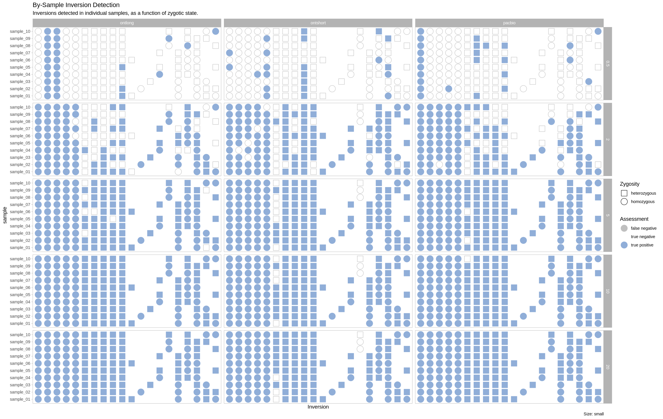
We are plotting the inversions across the genome as a visual assessment, along with a presence/absence matrix across platforms and zygotic state. Small inversions were made bigger by 100kb to see them easier on the plot. All other inversions had their lengths increased by 50kb for the same reason.

plot_inversions <- function(data, size_treatment){
    if(size_treatment == "small"){
        scale_factor = 100000
    } else {
        scale_factor = 50000
    }

    filter(data, size == size_treatment, assessment == "true positive") %>%
    ggplot(
        aes(
            x = sample,
            ymin = position_start,
            ymax = position_end + scale_factor,
            color = platform,
        )
    ) +
        scale_y_continuous(labels = scales::comma) +
        coord_flip() +
        geom_linerange(position = position_dodge(.7), linewidth = 2) +
        labs(title = "Called Inversions Across the Genome", subtitle = paste0("Size: ", size_treatment), y = "genomic position (bp)") + 
        facet_grid(cols = vars(contig), rows = vars(depth)) +
        theme_light() +
        theme(panel.grid.major.y = element_blank(), legend.position = "top")
}

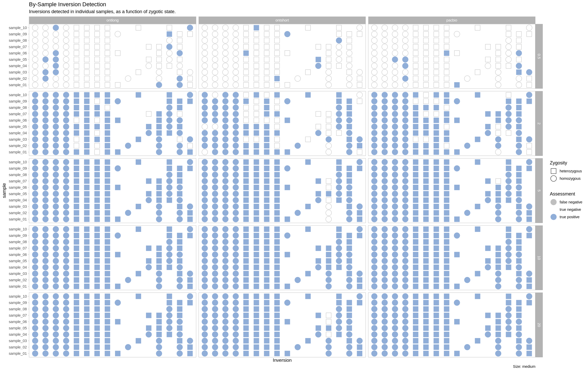
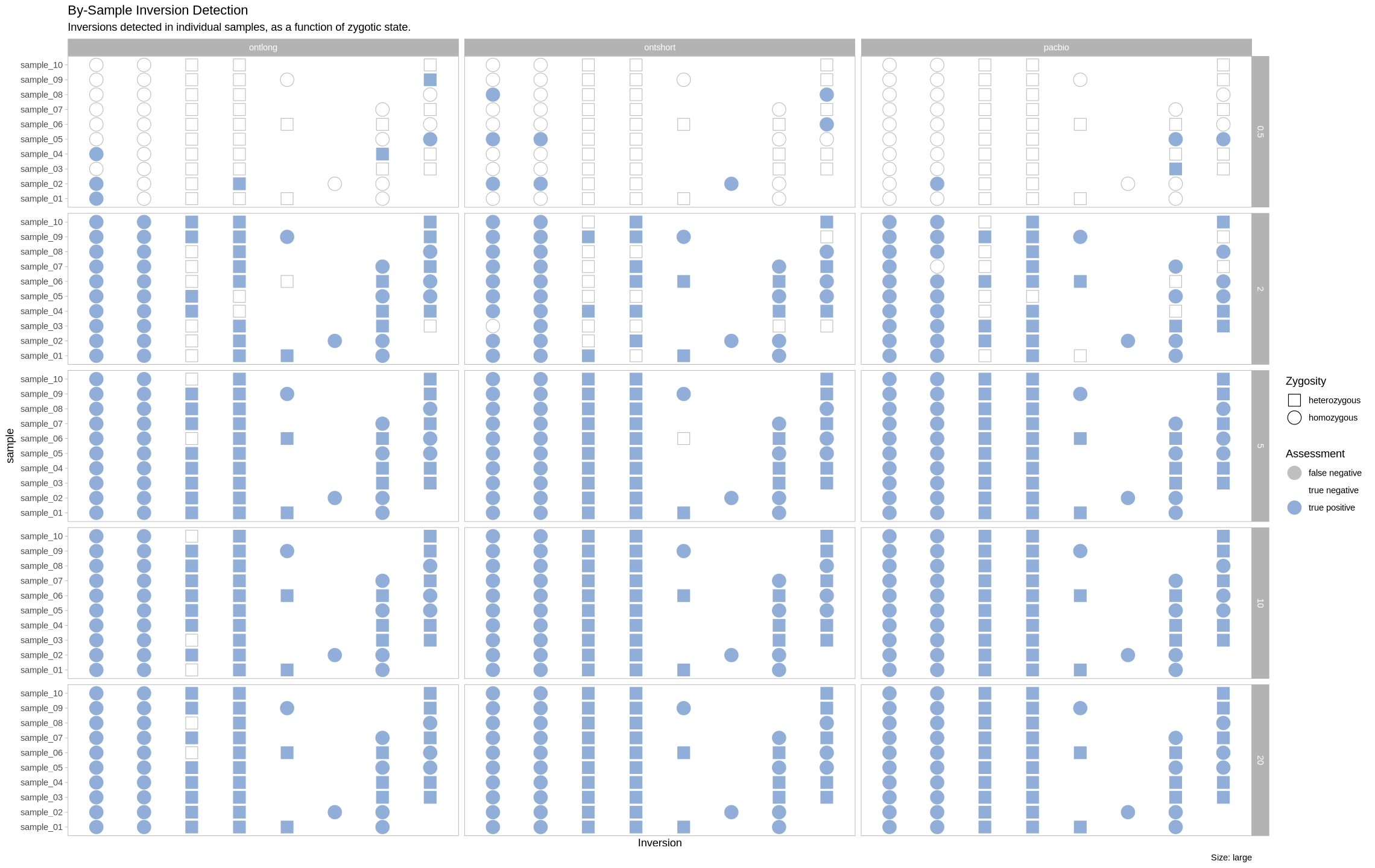
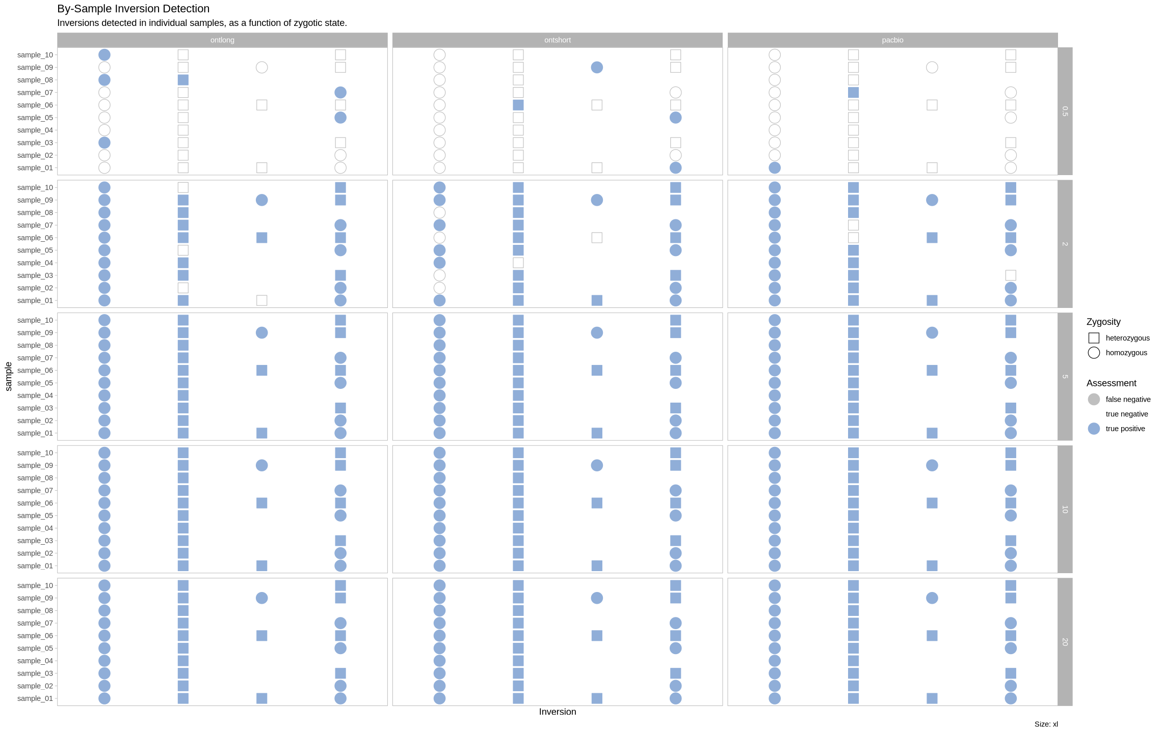
plot_samples_matrix <- function(data, size_treatment){
filter(data, size == size_treatment) %>%
    group_by(size, contig, position_start) %>% mutate(id = cur_group_id()) %>% ungroup() %>%
    ggplot(aes(y = sample, x = id, fill = assessment, color = assessment, shape = zygosity)) +
        geom_point(size=6) +
        theme_light() +
        labs(title = "By-Sample Inversion Detection", subtitle = "Inversions detected in individual samples, as a function of zygotic state.", caption = paste0("Size: ", size_treatment)) +
        scale_color_manual(name = "Assessment", values = c("false negative" = "grey75", "true negative" = "white", "true positive" = "#90aed8")) +
        scale_fill_manual(name = "Assessment", values = c("false negative" = "white", "true negative" = "white", "true positive" = "#90aed8")) +
        scale_shape_manual(name = "Zygosity", values = c("homozygous" = 21, "heterozygous" = 22)) +
        scale_x_discrete(name = "Inversion") +
        theme(
            panel.grid.major = element_blank(),
            panel.grid.minor = element_blank()
        ) +
        facet_grid(rows = vars(depth), cols = vars(platform))
}

Small Inversions¶

plot_inversions(assessment_df, "small")
plot_samples_matrix(assessment_df, "small")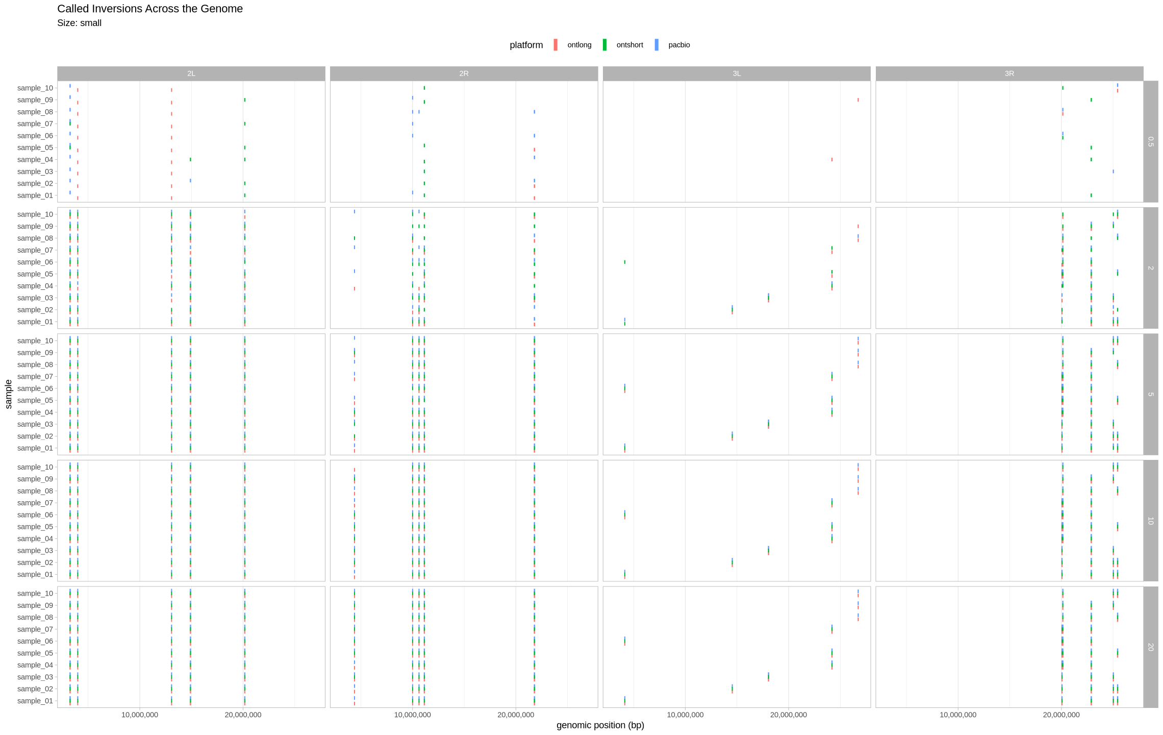

Medium Inversions¶

plot_inversions(assessment_df, "medium")
plot_samples_matrix(assessment_df, "medium")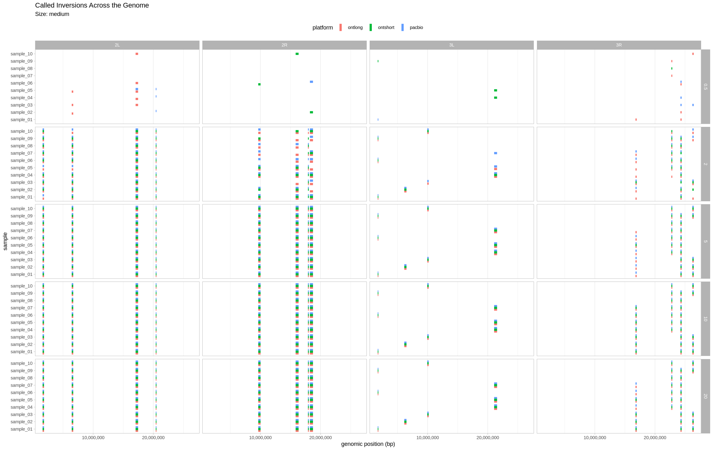

Large Inversions¶

plot_inversions(assessment_df, "large")
plot_samples_matrix(assessment_df, "large")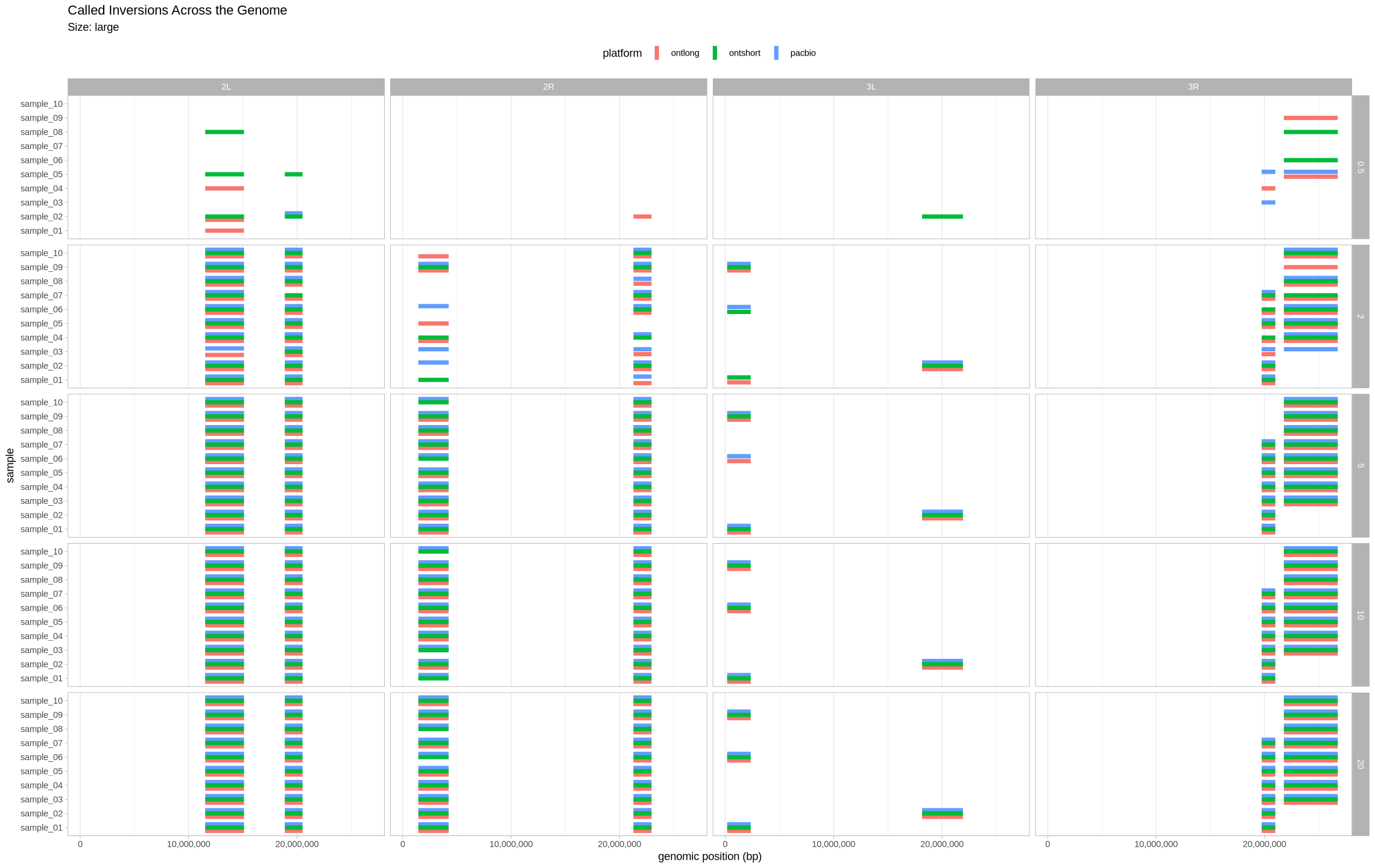

XL Inversions¶

plot_inversions(assessment_df, "xl")
plot_samples_matrix(assessment_df, "xl")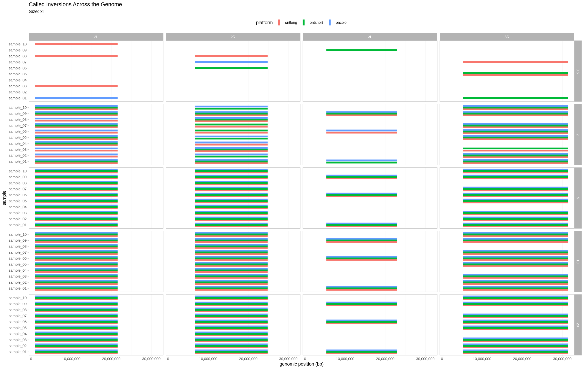

Precision vs Recall¶

metrics <- group_by(assessment_df, size, depth, platform) %>%
    summarize(
        TP = sum(assessment == "true positive"),
        FP = sum(assessment == "false positive"),
        TN = sum(assessment == "true negative"),
        FN = sum(assessment == "false negative")
    ) %>% ungroup()
metrics$precision <- metrics$TP / (metrics$TP + metrics$FP)
metrics$recall <- metrics$TP / (metrics$TP + metrics$FN)
metrics$F1 <- 2 * ((metrics$precision * metrics$recall) / (metrics$precision + metrics$recall))
metrics$depth <- metrics$depth
metrics$size <- factor(metrics$size, ordered = T, levels = c("small", "medium", "large", "xl"))
head(metrics)

`summarise()` has grouped output by 'size', 'depth'. You can override using the
`.groups` argument.

greys <- c(
    "#c0c6cf",
    "#a2aab5",
    "#6e7684",
    "#54546c",
    "black"
)

colorful <- c(
    "#9b6981",
    "#682c37",
    "#f6955e" ,
    "#a8cdec"
)

options(warn = -1, repr.plot.width = 10, repr.plot.height = 10)
ggplot(metrics, aes(x = recall, y = precision, color = as.factor(depth), shape = size)) +
    geom_abline(intercept = 0, slope = 1, color = "#ab99b1ff") +
    geom_point(size = 6) +
    theme_light() +
    scale_color_manual(name = "Sample Depth", values = greys) +
    scale_shape_manual(name = "Inversion Size", values = c(19,15,18,17)) +
    coord_cartesian(xlim = c(0,1), ylim = c(0,1)) +
    labs(title = "Precision-Recall Curve (long reads)") +
    facet_grid(cols = vars(platform), rows = vars(size))

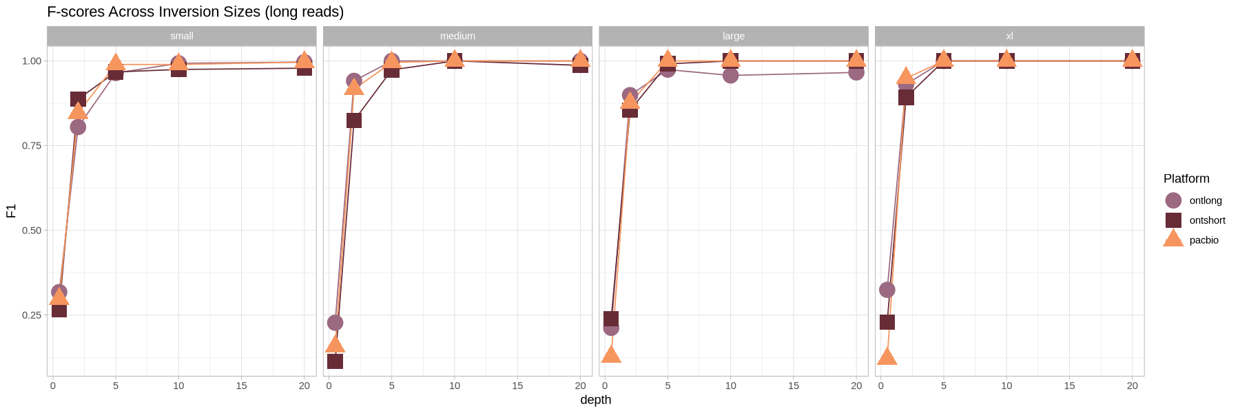
options(warn = -1, repr.plot.width = 15, repr.plot.height = 5)
ggplot(metrics, aes(x = depth, y = F1, color = platform, shape = platform, group = paste(size, platform))) +
    geom_line() +
    geom_point(size = 6) +
    theme_light() +
    scale_shape_manual(name = "Platform", values = c(19, 15, 17)) +
    scale_color_manual(name = "Platform", values = colorful) +
    labs(title = "F-scores Across Inversion Sizes (long reads)") +
    facet_grid(cols = vars(size))