Small Inversions - Inversion Simulations

Here, we visualize the inversions that were identified for the small treatment across the range of depths. The LEVIATHAN small, medium, and large call rates are configured to -s 95 -m 95 -l 90.

library(ggplot2)
library(ggpattern)
library(dplyr)
library(ggpubr)
.size <- "small"


Attaching package: 'dplyr'


The following objects are masked from 'package:stats':

    filter, lag


The following objects are masked from 'package:base':

    intersect, setdiff, setequal, union

These are the setup functions that process that data.

read_data <- function(size_treatment, depth){
    .depth <- paste("depth",depth, sep = "_")
    truthfile <- paste0("simulated_variants/setup_inversions/", size_treatment, "/inv.", size_treatment,".vcf")
    samplesfile <- paste("simulated_data/called_sv/leviathan", size_treatment, .depth, "by_sample90/inversions.bedpe", sep = "/")
    poolfile <- paste("simulated_data/called_sv/leviathan", size_treatment, .depth, "by_pop90/inversions.bedpe", sep = "/")

    true_inversions <- read.table(truthfile, header = F)[,c(1,2,8)]
    true_inversions$V8 <- as.numeric(unlist(lapply(true_inversions$V8, function(X){gsub(".+END=", "", X)})))
    names(true_inversions) <- c("contig", "position_start", "position_end")
    true_inversions$sample <- "simulated_inversions"

    sample_inversions <- read.table(samplesfile, header = T)[,1:4]

    pooled_inversions <- read.table(poolfile, header = T)
    pooled_inversions <- pooled_inversions[,c("population","contig", "position_start", "position_end")]
    names(pooled_inversions)[1] <- "sample"
    if( nrow(pooled_inversions) > 0){
        pooled_inversions$sample <- "pooled" #paste("pooled", depth, size_treatment, sep = "_")
    }
    outdf <- rbind(true_inversions, sample_inversions, pooled_inversions)
    outdf$depth <- depth
    return(outdf)
}

read_all_data <- function(size_treatment){
    depth <- 0.5
    .data <- read_data(size_treatment, depth)    
    for(i in c(2,5,10,20)){
        .data <- rbind(.data, read_data(.size, i))    
    }
    return(.data)
}

SV <- read_all_data("large")
samplesSV <- SV[SV$sample != "simulated_inversions",]
head(samplesSV)

A function to wrap all these other functions for simplicity.

summarize_performance <- function(inventory, .size){
    depth <- 0.5
    .data <- read_data(.size, depth)    
    for(i in c(2,5,10,20)){
        .data <- rbind(.data, read_data(.size, i))    
    }
    .performance <- assess_performace(.data, inventory)
    .sampleplot <- plot_samples_matrix(.performance, .size)
    .poolplot <- plot_pools_matrix(.performance, .size)
    .inversionplot <- plot_inversions(.data, .size)
    show(
        ggarrange(
            ggarrange(.sampleplot, .poolplot, ncol = 2, labels = c("A", "B"), common.legend = T),
            .inversionplot, nrow = 2, labels = c("","C"), heights = c(1.5,4)
        )
    )
    return(.performance)
}

Read in the sample and pool simulation inventory

inventory <- rbind(
    filter(read.table("inversion_simulations.inventory", header = T), size == .size),
    filter(read.table("inversion_simulations.pool.inventory", header = T), size == .size)
)
inventory <- rename(inventory, "simulated" = "present", "zygosity" = "state")

# set a default to false negatives, to be updated to true positives when conditions are met
inventory$assessment <- ifelse(inventory$simulated, "false negative", "true negative")
inventory$sample <- gsub("pool", "pooled", inventory$sample)

# add depths to performance
# arrange() is for sanity-checking
performance <- inventory
performance$depth <- 0.5
for(i in c(2, 5, 10, 20)){
    inventory$depth <- i
    performance <- rbind(performance, inventory)
}
performance <- arrange(performance, sample, contig, inversion)

## read in truth data to transfer inversion breakpoints
x <- read_data(.size, 0.5)
for(i in c(2,5,10,20)){
    x <- rbind(x, read_data(.size, i))
}
x <- arrange(x, sample, contig, position_start, depth)

truth <- group_by(x[x$sample == "simulated_inversions",], contig, depth) %>% mutate(inversion = 1:n()) %>% ungroup()
truth <- truth[, c(1,6,2,3,5)]

# merge it all together
performance <- merge(performance,truth, by = c("contig", "inversion", "depth"))
performance$id <- as.integer(as.factor(performance$position_start))
performance <- arrange(performance[, c(1,2,11,3,4:10)], contig, inversion, sample, depth)
head(performance, 15)

Assess the performance of identified inversions¶

false_positives <- samplesSV[0,]

for(i in 1:nrow(samplesSV)){
    .row <- samplesSV[i,]
    query <- which(
        performance$sample == .row$sample &
        performance$depth == .row$depth &
        performance$contig == .row$contig &
        performance$position_start - 50 <= .row$position_start &
        performance$position_end + 50 >= .row$position_end
    )
    if(length(query) > 0 && performance$simulated[query]){
        performance$assessment[query] <- "true positive"
    } else {
        performance$assessment[query] <- "false positive"
        false_positives <- rbind(false_positives, .row)
    }
}
head(performance)
head(false_positives)

This is extra formatting we need to do to get it to plot correctly

performance$sample <- gsub("sample_", "", performance$sample)
performance$sample <- gsub("pooled", "11", performance$sample)
performance$sample <- as.integer(performance$sample)

simulated_for_plot <- truth
simulated_for_plot$assessment <- "true positive"
simulated_for_plot$sample <- 0
simulated_for_plot <- simulated_for_plot[simulated_for_plot$depth == 20,]
head(simulated_for_plot)

Single-Sample Detection¶

Let’s first visualize what detection looked like across the genome. Here, we facet across contigs and show all the depths at once. Since the small inversions are indeed quite small, for visualization purposes, we’ll make each of them 100 kb bigger.

plot_inversions <- function(data, groundtruth, size_treatment){
    options(warn = -1, repr.plot.width = 19, repr.plot.height = 10)
    .tbl <- filter(data, assessment == "true positive") %>% select(contig, inversion, position_start, position_end, depth, assessment, sample)
    
    rbind(.tbl, groundtruth) %>%

    ggplot(
        aes(
            x = sample,
            ymin = position_start,
            ymax = position_end+100000,
            color = as.factor(depth),
        )
    ) +
        geom_linerange(position = position_dodge(0.7), linewidth = 1.5) +
        coord_flip() +
        scale_color_brewer(name = "sequencing depth", palette = "Set2") +
        scale_x_continuous(breaks = 0:11,limits = c(0, 11)) +
        scale_y_continuous(labels = scales::comma) +
        theme_light() +
        theme(
            panel.grid.major.y = element_blank(),
            legend.position = "top",
            panel.grid.minor.y = element_line(color = "gray80", size = 0.5)
        ) +
        labs(
            title = "Simulated and Called Inversions Across the Genome",
            subtitle = paste0("Size: ", size_treatment),
            y = "genomic position (bp)",
            caption = "sample 0 = groundtruth | sample 11 = pooled"
        ) + 
        facet_grid(cols = vars(contig))
}

plot_inversions(performance, simulated_for_plot, .size)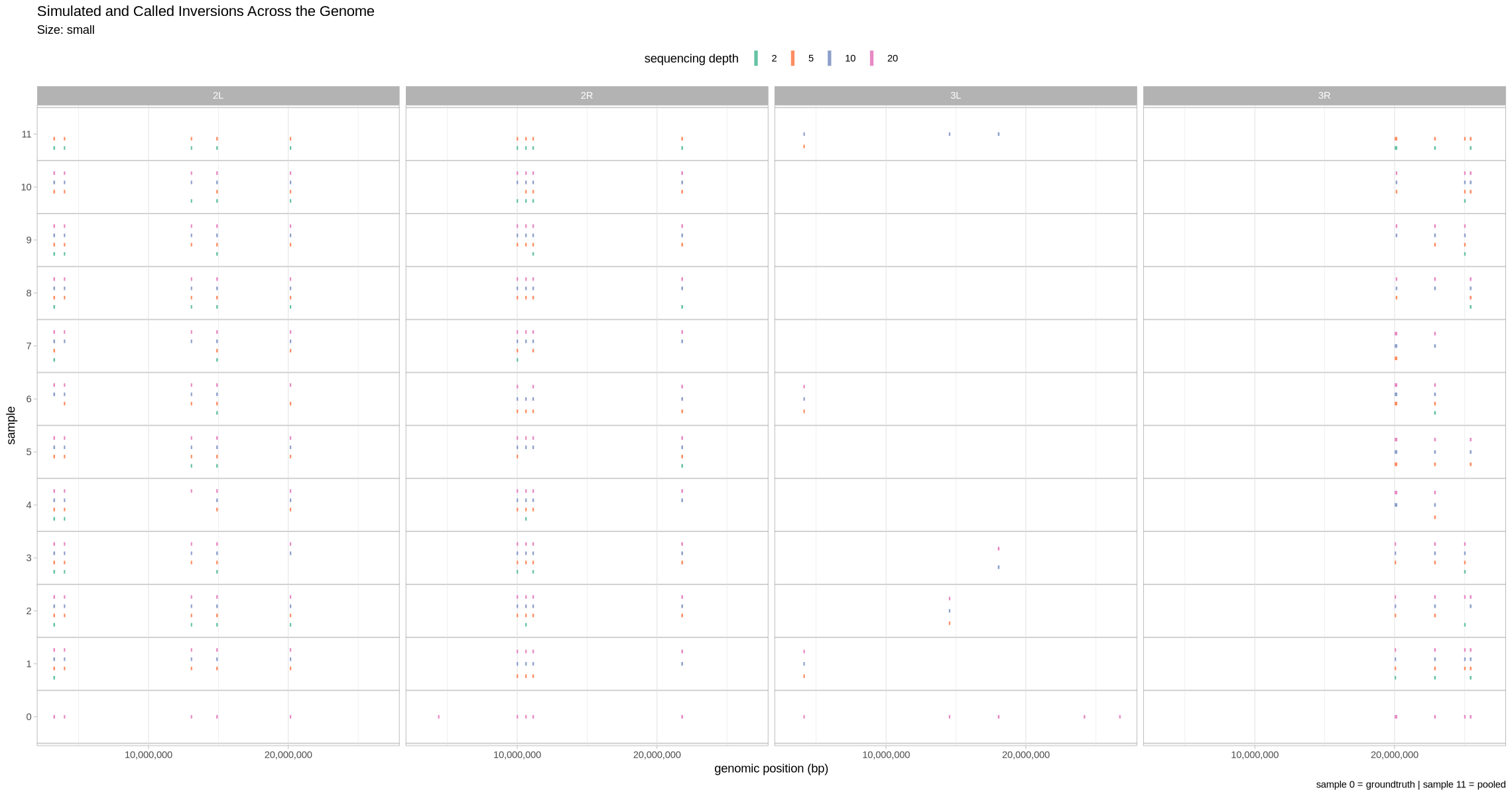

What does this look like as a heatmap of true/false positive/negative?

plot_samples_matrix <- function(data, size_treatment){
    options(warn = -1, repr.plot.width = 10, repr.plot.height = 15)
    .data <- data[data$sample != 11,]
    axis_ticks <- factor(paste0("sample_", sprintf("%02d", 1:10)))
    ggplot(.data, aes(y = sample, x = id, fill = assessment, pattern = zygosity)) +
        geom_tile_pattern(
            pattern_color = NA,
            color = "white",
            pattern_fill = "black",
            pattern_angle = 45,
            pattern_density = 0.5,
            pattern_spacing = 0.025,
            pattern_key_scale_factor = 1
        ) +
        theme_light() +
        labs(title = "By-Sample Inversion Detection", subtitle = paste(size_treatment, "inversions detected in individual samples, as a function of zygotic state.")) +
        scale_fill_manual(values = c("false negative" = "#eaf398ff", "true negative" = "grey70", "true positive" = "#90aed8")) +
        scale_pattern_manual(values = c("het" = "circle", "hom" = "none")) +
        scale_x_discrete(name = "Inversion") +
        scale_y_discrete(limits = axis_ticks, breaks = axis_ticks) +
        coord_cartesian(xlim = c(1, max(data$id)), expand = F) +
        theme(
            panel.grid.major = element_blank(),
            panel.grid.minor = element_blank()
        ) +
        facet_grid(rows = vars(depth))
}

plot_samples_matrix(performance, .size)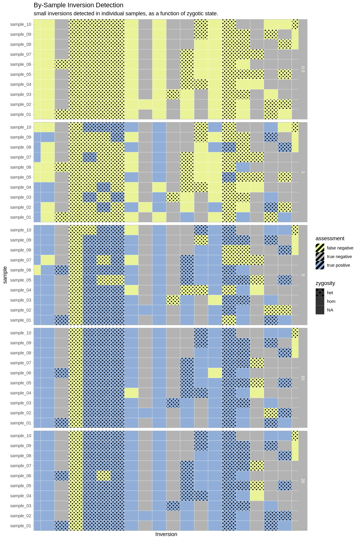

Pooled Sample Detection¶

plot_pools_matrix <- function(data, size_treatment){
    options(warn = -1, repr.plot.width = 15, repr.plot.height = 10)
    .data <- data[data$sample == 11,]
    .data$contig <- gsub("2L", "2L (all homozygous)", .data$contig)
    .data$contig <- gsub("2R", "2R (all heterozygous)", .data$contig)
    .data$contig <- gsub("3L", "3L (inversions common)", .data$contig)
    .data$contig <- gsub("3R", "3R (inversions rare)", .data$contig)
 
    ggplot(.data, aes(y = 1, x = inversion, fill = assessment)) +
        geom_tile(color = "white", linewidth = 1.5) +
        theme_light() +
        labs(title = "Pooled-Sample Detection", subtitle = paste(size_treatment, "inversions detected in sample-pooled data, as a function of inversion frequency in the population.")) +
        scale_fill_manual(values = c("false negative" = "grey70", "true positive" = "#90aed8")) +
        scale_y_continuous(breaks = 1, name = "Assessment") +
        scale_x_discrete(name = "Inversion") +
        theme(
            panel.grid.major = element_blank(),
            panel.grid.minor = element_blank(),
            axis.text.y = element_blank(),
            axis.ticks.y = element_blank()
        ) +
        coord_cartesian(xlim = c(1, max(data$inversion)), expand = F) +
        facet_grid(cols = vars(contig), rows = vars(depth))
}

plot_pools_matrix(performance, .size)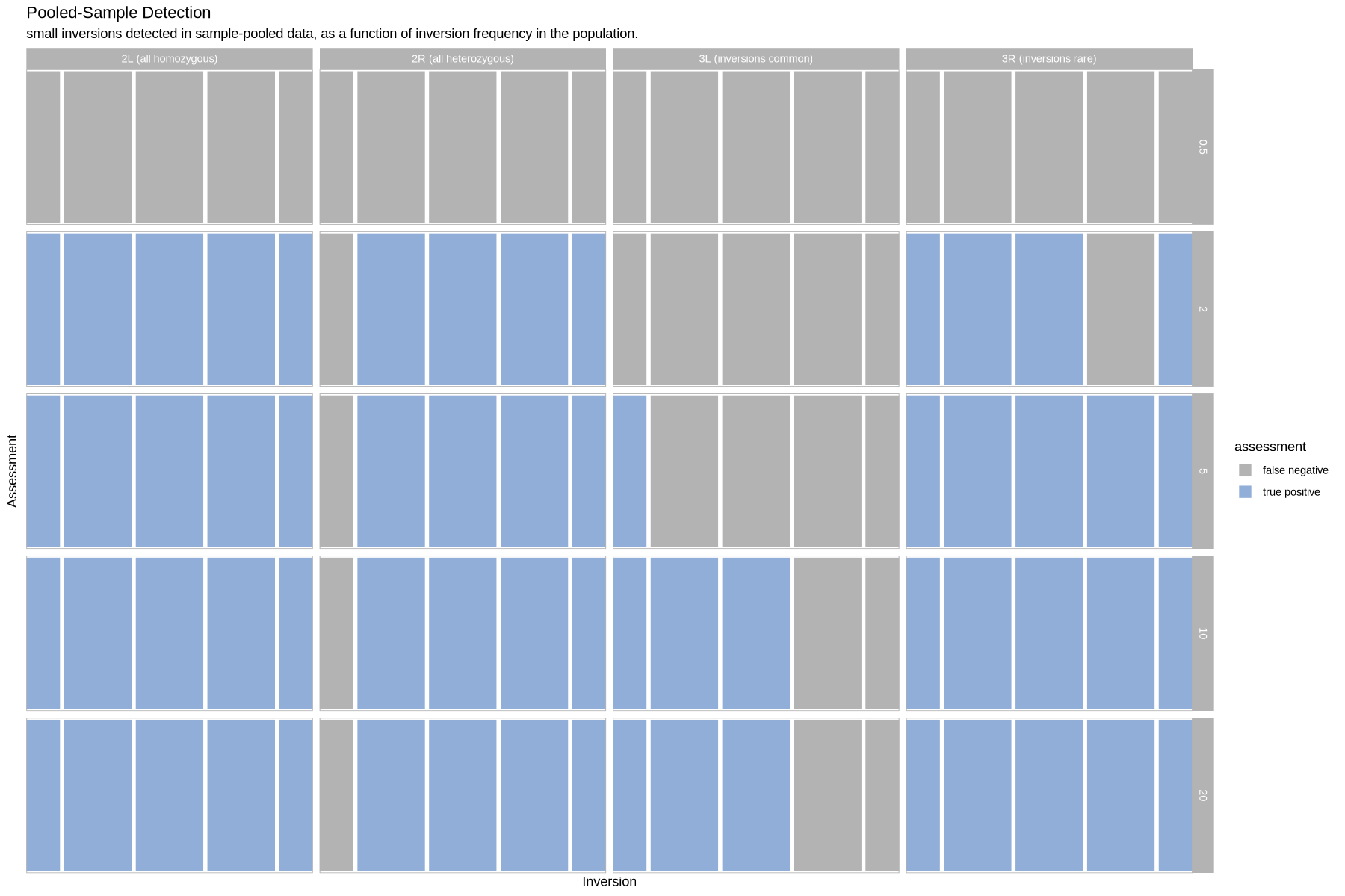

Write this all to a file to tease apart later

ifelse(!dir.exists("assess_called_sv"), dir.create("assess_called_sv"), TRUE)
write.csv(performance, file = paste0("assess_called_sv/",.size, ".sv.assessment"), quote = F, row.names = F)

04a Check called inversions (by size)

Compare Inversion Calls Across Treatments

04a Check called inversions (by size)

Medium Inversions