Are inversions in repeat regions? - Inversion Simulations

Now that we did some repeat modeling and classification, we can see if the breakpoints of any of the simulated inversions fall into these identified repeat regions.

library(dplyr)
library(ggplot2)
library(ggh4x)
library(tidyr)

Read in the repeat data¶

repeats <- read.table("repeat.regions", header = T)
repeats <- arrange(repeats[order(repeats$contig), ], contig, position_start)
# overwrite the file with it being sorted by chrom + start position
#write.table(repeats, file = "repeat.regions", quote = F, row.names = F)
nrow(repeats)
head(repeats, 15)

Read in inversion inventory¶

We’ll to read in the inventory of all inversion positions and pull out the unique inversions. I really should have committed to either comma or tab separated tables.

inversions <- read.csv("../assess_called_sv/linkedread.sv.assessment", header = T)
inversions <- unique(inversions[, c(1,6,10,11)])
rownames(inversions) <- NULL
inversions$is_repeat <- as.character(NA)
inversions$which_breakpoints <- 0
inversions$is_repeat_start <- as.character(NA)
inversions$is_repeat_end <- as.character(NA)
head(inversions)

Assess which inversions are in or adjacent to repeat regions¶

To do the matchy-matchy, similar to what we did to assess inversion calling. It will need some modifications to accommodate the slightly different use case. Primarily, adding a 800bp buffer to the repeat breakpoints to catch inversion breakpoints that might be within an insert-size of the repeat breakpoint.

for(i in 1:nrow(inversions)){
    .row <- inversions[i,]
    # first breakpoint
    query <- which(
        repeats$contig == .row$contig &
        (repeats$position_start - 800 <= .row$position_start & repeats$position_end + 800 >= .row$position_start)
    )
    if(length(query) > 0) {
        inversions$is_repeat_start[i] <- paste(repeats$class[query], collapse = ";")
        inversions$which_breakpoints[i] <- inversions$which_breakpoints[i] + 1  
    }
    # second breakpoint
    query <- which(
        repeats$contig == .row$contig &
        (repeats$position_start - 800 <= .row$position_end) & (repeats$position_end + 800 >= .row$position_end)
    )
    if(length(query) > 0) {
        inversions$is_repeat_end[i] <- paste(repeats$class[query], collapse = ";")
        inversions$which_breakpoints[i] <- inversions$which_breakpoints[i] + 2
    }
}
inversions$is_repeat <- !is.na(inversions$is_repeat_start) | !is.na(inversions$is_repeat_end)
are_repeats <- inversions[inversions$is_repeat,]
are_repeats

Read in inversion results¶

Let’s find which inversions had the most false negatives.

called_sv <- read.csv("../assess_called_sv/linkedread.sv.assessment", header = T)
false_neg <- group_by(called_sv, contig, position_start, size) %>%
    mutate(perc = round(sum(assessment == "false negative")/length(depth) * 100,1)) %>%
    filter(assessment == "false negative") %>%
    summarize(n = length(depth), perc = unique(perc)) %>%
    ungroup() %>%
    arrange(desc(n))

false_neg$is_repeat <- FALSE
false_neg$which_breakpoint <- as.integer(0)
head(false_neg)

We can now combine the inversions-in-repeats with the inversions-not-detected dataframe to see if there’s a correlation of hard-to-call inversions being associated with repeat regions.

for(i in 1:nrow(false_neg)){
    .row <- false_neg[i,]
    query <- which(
        are_repeats$contig == .row$contig &
        are_repeats$position_start == .row$position_start
    )
    if(length(query) > 0) {
        false_neg$is_repeat[i] <- TRUE
        false_neg$which_breakpoint[i] <- are_repeats$which_breakpoints[query]
    }
}
false_neg$platform <- "linkedread"
head(arrange(false_neg, desc(is_repeat)))

For comparison sake, we need to do this with the long-read inversion detections as well. We’ll read it in and extract only the relevant columns and only rows where assessment is false negative.

long_inv <- read.csv("../longread_workflow/longread.sv.assessment", header = T)
false_neg_long <- group_by(long_inv[,c(2:5, 8,10)], contig, position_start, size, platform) %>%
    mutate(perc = round(sum(assessment == "false negative")/length(assessment) * 100,1)) %>%
    filter(assessment == "false negative") %>%
    summarize(n = length(assessment), perc = unique(perc)) %>%
    ungroup() %>%
    arrange(desc(n))
false_neg_long$is_repeat <- FALSE
false_neg_long$which_breakpoint <- as.integer(0)

head(false_neg_long, 20)

Now do the same matching between inversions and repeat regions

for(i in 1:nrow(false_neg_long)){
    .row <- false_neg_long[i,]
    query <- which(
        are_repeats$contig == .row$contig &
        are_repeats$position_start == .row$position_start
    )
    if(length(query) > 0) {
        false_neg_long$is_repeat[i] <- TRUE
        false_neg_long$which_breakpoint[i] <- are_repeats$which_breakpoint[query]
    }
}
head(arrange(false_neg_long, desc(is_repeat)))

Let’s combine the two dataframes so we can start plotting them to meaningfully represent these data. This will also include making platform, size, and contig ordered factors.

false_neg_all <- rbind(false_neg, false_neg_long) %>% arrange(desc(n), desc(platform), desc(size))
false_neg_all$contig <- factor(false_neg_all$contig, levels = c("2L", "2R","3L","3R"), ordered = T)
false_neg_all$size <- factor(false_neg_all$size, levels = c("small", "medium", "large", "xl"))
false_neg_all$platform <- factor(false_neg_all$platform, levels = c("linkedread","ontshort","ontlong","pacbio"))

head(false_neg_all)

It may be worth adding a column of unique identifiers for the inversions for plotting purposes.

false_neg_all <- group_by(false_neg_all, is_repeat,position_start) %>%
    mutate(inv_id = cur_group_id())
false_neg_all$seq_id <- 1:nrow(false_neg_all)
head(false_neg_all, 15)

Visualization¶

tech_colors <- c(
    "ontshort" = "#9b6981",
    "ontlong" = "#682c37",
    "pacbio" = "#f6955e" ,
    "linkedread" = "#a8cdec"
)

size_colors <- c(
    "#c0c6cf",
    "#a2aab5",
    "#6e7684",
    "#54546c"
)

options(repr.plot.width = 20, repr.plot.height = 8)
ggplot(false_neg_all, aes(x = seq_id, y = 0, yend = perc, shape = size, color = platform)) +
    geom_point(size = 4, aes(y = perc)) +
    geom_segment(aes(linetype = is_repeat), linewidth = 1.1) +
    theme_light() +
    scale_shape_manual(values = c(19,15,18,17)) +
    scale_color_manual(values = tech_colors) +
    coord_cartesian(xlim = c(-2, 195), ylim = c(0, 101),expand = F) +
    labs(
        title = "False Positives in Repeat Regions",
        color = "Technology",
        shape = "Inversion Size",
        linetype = "In Repeat Region"
    ) +
    theme(
        axis.text.x=element_blank(),
        axis.ticks.x=element_blank()
    ) +
    xlab("Inversion") +
    ylab("Percent False Positive Detection Across Samples")

options(repr.plot.width = 20, repr.plot.height = 8)
.strip <- strip_themed(background_y = elem_list_rect(fill = tech_colors))

false_neg_all %>% group_by(platform) %>% 
    mutate(mx = max(perc)) %>% 
    arrange(desc(mx), .by_group = T) %>% 
    mutate(id = 1:length(perc)) %>%
    ggplot(aes(x = id, y = 0, yend = perc, shape = size, color = size)) +
        geom_point(size = 6, aes(y = perc)) +
        geom_segment(aes(linetype = is_repeat), linewidth = 2) +
        theme_light() +
        scale_shape_manual(values = c(19,15,18,17)) +
        scale_color_manual(values = size_colors) +
        labs(
            title = "False Positives in Repeat Regions",
            color = "Inversion Size",
            shape = "Inversion Size",
            linetype = "In Repeat Region"
        ) +
        theme(
            axis.text.x=element_blank(),
            axis.ticks.x=element_blank()
        ) +
        xlab("Inversion") +
        ylab("Percent False Positive Detection Across Samples") +
        facet_grid2(rows = vars(platform), strip = .strip)

options(repr.plot.width = 20, repr.plot.height = 8)
.strip <- strip_themed(background_y = elem_list_rect(fill = size_colors))

false_neg_all %>% group_by(size) %>% 
    mutate(mx = max(perc)) %>% 
    arrange(desc(mx), .by_group = T) %>% 
    mutate(id = 1:length(perc)) %>%
    ggplot(aes(x = id, y = 0, yend = perc, shape = platform, color = platform)) +
        geom_point(size = 5, aes(y = perc)) +
        geom_segment(aes(linetype = is_repeat), linewidth = 1.5) +
        theme_light() +
        scale_shape_manual(values = c(19,15,18,17)) +
        scale_color_manual(values = tech_colors) +
        labs(
            title = "False Positives in Repeat Regions",
            color = "Technology",
            shape = "Technology",
            linetype = "In Repeat Region"
        ) +
        theme(
            axis.text.x=element_blank(),
            axis.ticks.x=element_blank()
        ) +
        xlab("Inversion") +
        ylab("Percent False Positive Detection Across Samples") +
        facet_grid2(rows = vars(size), scales = "free_x", independent = "x", strip = .strip)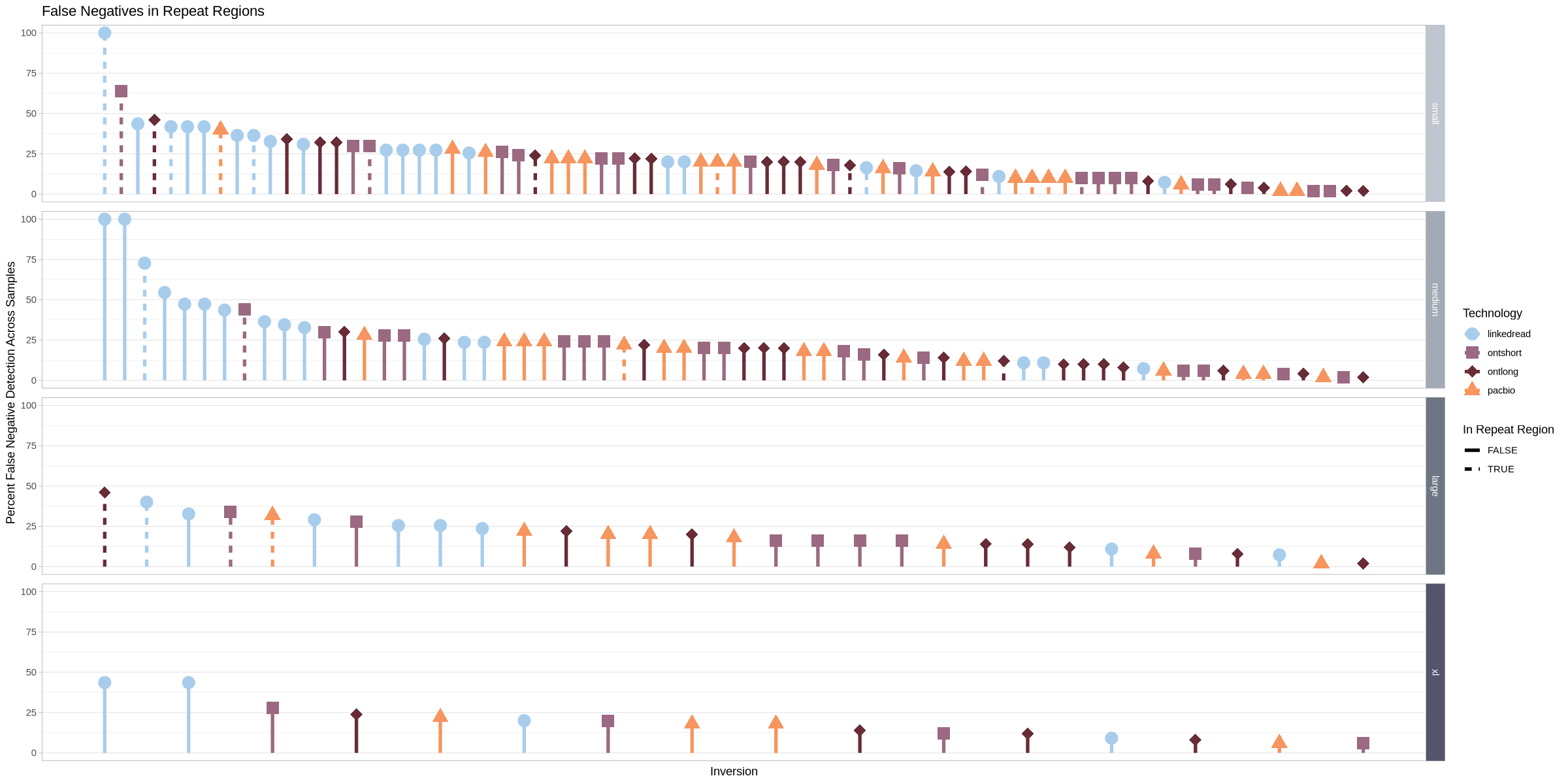

freq_colors <- c(
    "#a4c0d8ff",
    "#a86cafff"
)
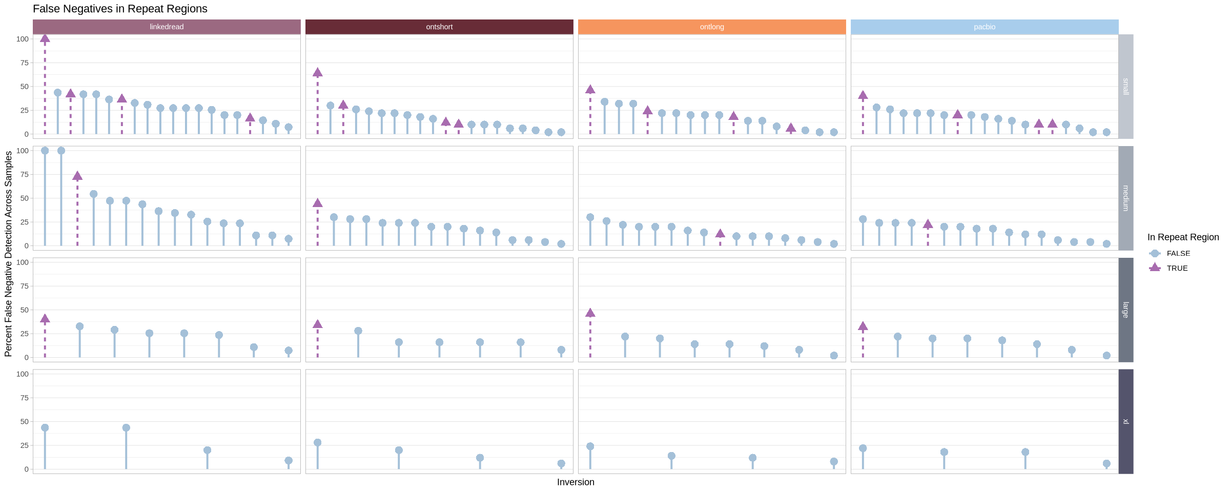
options(repr.plot.width = 20, repr.plot.height = 8)
.strip <- strip_themed(background_x = elem_list_rect(fill = tech_colors), background_y = elem_list_rect(fill = size_colors))

false_neg_all %>% group_by(platform, size) %>% 
    mutate(mx = max(perc)) %>% 
    arrange(desc(mx), .by_group = T) %>% 
    mutate(id = 1:length(perc)) %>%
    ggplot(aes(x = id, y = 0, yend = perc, shape = is_repeat, color = is_repeat)) +
        geom_point(size = 4, aes(y = perc)) +
        geom_segment(aes(linetype = is_repeat), linewidth = 1.1) +
        theme_light() +
        #scale_shape_manual(values = c(19,15,18,17)) +
        scale_color_manual(values = freq_colors) +
        labs(
            title = "False Positives in Repeat Regions",
            color = "In Repeat Region",
            shape = "In Repeat Region",
            linetype = "In Repeat Region"
        ) +
        theme(
            axis.text.x=element_blank(),
            axis.ticks.x=element_blank()
        ) +
        xlab("Inversion") +
        ylab("Percent False Positive Detection Across Samples") +
        facet_grid2(rows = vars(size), cols = vars(platform), scales = "free_x", independent = "x", strip = .strip)

Inversion sanity checks

Repeat Modeling

Inversion sanity checks

Did LEVIATHAN filter the inversions?