Here, we visualize the inversions that were identified for the small treatment across the range of depths. The LEVIATHAN small, medium, and large call rates are configured to -s 90 -m 90 -l 90.
library(ggplot2)
library(dplyr)
library(ggpubr)
.size <- "small"
Output
Attaching package: 'dplyr'


The following objects are masked from 'package:stats':

    filter, lag


The following objects are masked from 'package:base':

    intersect, setdiff, setequal, union
These are the setup functions that process that data.
Source
read_data <- function(size_treatment, depth){
    .depth <- paste("depth",depth, sep = "_")
    samplesfile <- paste("../../simulated_data/visor/called_sv/leviathan", size_treatment, .depth, "by_sample/inversions.bedpe", sep = "/")
    poolfile <- paste("../../simulated_data/visor/called_sv/leviathan", size_treatment, .depth, "by_pop/inversions.bedpe", sep = "/")

    sample_inversions <- read.table(samplesfile, header = T)[,1:4]
    sample_inversions$sample <- as.integer(gsub("sample_", "", sample_inversions$sample))
    pooled_inversions <- read.table(poolfile, header = T)
    pooled_inversions <- pooled_inversions[,c("population","contig", "position_start", "position_end")]
    names(pooled_inversions)[1] <- "sample"
    if( nrow(pooled_inversions) > 0){
        pooled_inversions$sample <- 11L
    }
    outdf <- rbind(sample_inversions, pooled_inversions)
    outdf$depth <- depth
    return(outdf)
}

read_candidatefile <- function(.size, .depth, .sample) {
    if (.sample <= 10){
        .cand_file <- sprintf("../../simulated_data/visor/called_sv/leviathan/%s/depth_%s/by_sample/logs/leviathan/sample_%02d.candidates", .size, .depth, .sample)
    } else {
        .cand_file <- sprintf("../../simulated_data/visor/called_sv/leviathan/%s/depth_%s/by_pop/logs/leviathan/pop1.candidates", .size, .depth)
    }
    .x <- read.table(
        .cand_file,
        col.names = c("contig", "position_start", "position_end", "contig2", "position_start2", "position_end2", "barcodes")
    )
    .x$sample <- .sample
    .x$depth <- .depth
    return (.x)
}

read_all_data <- function(size_treatment){
    .data <- read_data(size_treatment, 0.5)
    for(i in c(2,5,10,20)){
        .data <- rbind(.data, read_data(.size, i))
    }
    return(.data)
}
Read in all the leviathan candidates for this size inversion
# read in once to create properly formatted (but empty) table
candidates <- read_candidatefile(.size, 0.5, 1)[0,]

for (i in c(0.5, 2, 5, 10, 20)) {
    .depthcand <- Reduce(
        rbind,
        Map(function(x){read_candidatefile(.size, i, x)}, 1:11)
    )
    candidates <- rbind(candidates, .depthcand)
}

head(candidates)samplesSV <- read_all_data(.size)
head(samplesSV)Read in the sample and pool simulation inventory, add the assessment and candidate columns
Source
performance <- read.table("inversion.assessment", header = T)
performance <- performance[performance$size == .size,]
performance$assessment <- ifelse(performance$simulated, "false negative", "true negative")
performance$candidate <- F
head(performance)Assess the performance of identified inversions
near_breakpoint <- function(x, y, tolerance = 75){
    # x is the simulated/known breakpoints
    # y is the breakpoint we want to compare
    # check if y is within tolerance of x
    return(
        (y >= x - tolerance) & (y <= x + tolerance)
    )
}
false_positives <- samplesSV[0,]
for(i in 1:nrow(samplesSV)){
.row <- samplesSV[i,]
query <- which(
performance$sample == .row$sample &
performance$depth == .row$depth &
performance$contig == .row$contig &
near_breakpoint(performance$position_start, .row$position_start, 100) &
near_breakpoint(performance$position_end, .row$position_end, 100)
)
if(length(query) > 0) {
if (performance$simulated[query]){
performance$assessment[query] <- "true positive"
} else {
performance$assessment[query] <- "false positive"
false_positives <- rbind(false_positives, .row)
}
} # false negative otherwise
}
head(performance)Were false negatives ever initially detected in the candidates? In other words, did the first part of LEVIATHAN identify a potential inversion but filter it out after?
for(i in 1:nrow(performance)){
    if (performance$assessment[i] == "false negative"){
        # check if it's in the candidates
        .row <- performance[i,]
        query <- which(
            candidates$sample == .row$sample[1] &
            candidates$contig == .row$contig[1] &
            (.row$position_start[1]  > candidates$position_start & .row$position_start < candidates$position_end) &
            (.row$position_end[1]  > candidates$position_start2 & .row$position_end < candidates$position_end2)
        )
        if (length(query) > 0){
            performance$candidate[i] <- TRUE
        }
    }
}
head(performance[performance$candidate & performance$assessment == "false negative",])Create a column that looks for “not called but was a candidate”
performance$assess_cand <- gsub("false negative", "false negative (undetected)", performance$assessment)
performance$assess_cand[performance$assess_cand == "false negative (undetected)" & performance$candidate] <- "false negative (filtered)"
head(performance)Are there false positives?
head(false_positives)
if (nrow(false_positives) > 0) {
    false_positives$size <- .size
    false_positives$method <- "leviathan"
    write.table(false_positives, file = paste0("false_positives.", .size), row.names = F, quote = F)
}Augment the table to capture all the inversions that were simulated (groundtruth for plotting purposes)
truth <- filter(performance, simulated) %>%
    select(contig, inversion, position_start, position_end) |> unique() %>%
    mutate(assessment = "true positive", sample = 0, depth = 20)

head(truth)Single-Sample Detection
Let’s first visualize what detection looked like across the genome. Here, we facet across contigs and show all the depths at once. Since the small inversions are indeed quite small, for visualization purposes, we’ll make each of them 100 kb bigger.
Source
plot_inversions <- function(data, groundtruth, size_treatment){
    options(warn = -1, repr.plot.width = 19, repr.plot.height = 10)
    .tbl <- filter(data, assessment == "true positive") %>% select(contig, inversion, position_start, position_end, depth, assessment, sample)

    rbind(.tbl, groundtruth) %>%

    ggplot(
        aes(
            x = sample,
            ymin = position_start,
            ymax = position_end+100000,
            color = as.factor(depth),
        )
    ) +
        geom_linerange(position = position_dodge(0.7), linewidth = 1.5) +
        coord_flip() +
        scale_color_brewer(name = "sequencing depth", palette = "Set2") +
        scale_x_continuous(breaks = 0:11,limits = c(0, 11)) +
        scale_y_continuous(labels = scales::comma) +
        theme_light() +
        theme(
            panel.grid.major.y = element_blank(),
            legend.position = "top",
            panel.grid.minor.y = element_line(color = "gray80", size = 0.5)
        ) +
        labs(
            title = "Simulated and Called Inversions Across the Genome",
            subtitle = paste0("Size: ", size_treatment),
            y = "genomic position (bp)",
            caption = "sample 0 = groundtruth | sample 11 = pooled"
        ) +
        facet_grid(cols = vars(contig))
}
plot_inversions(performance, truth, .size)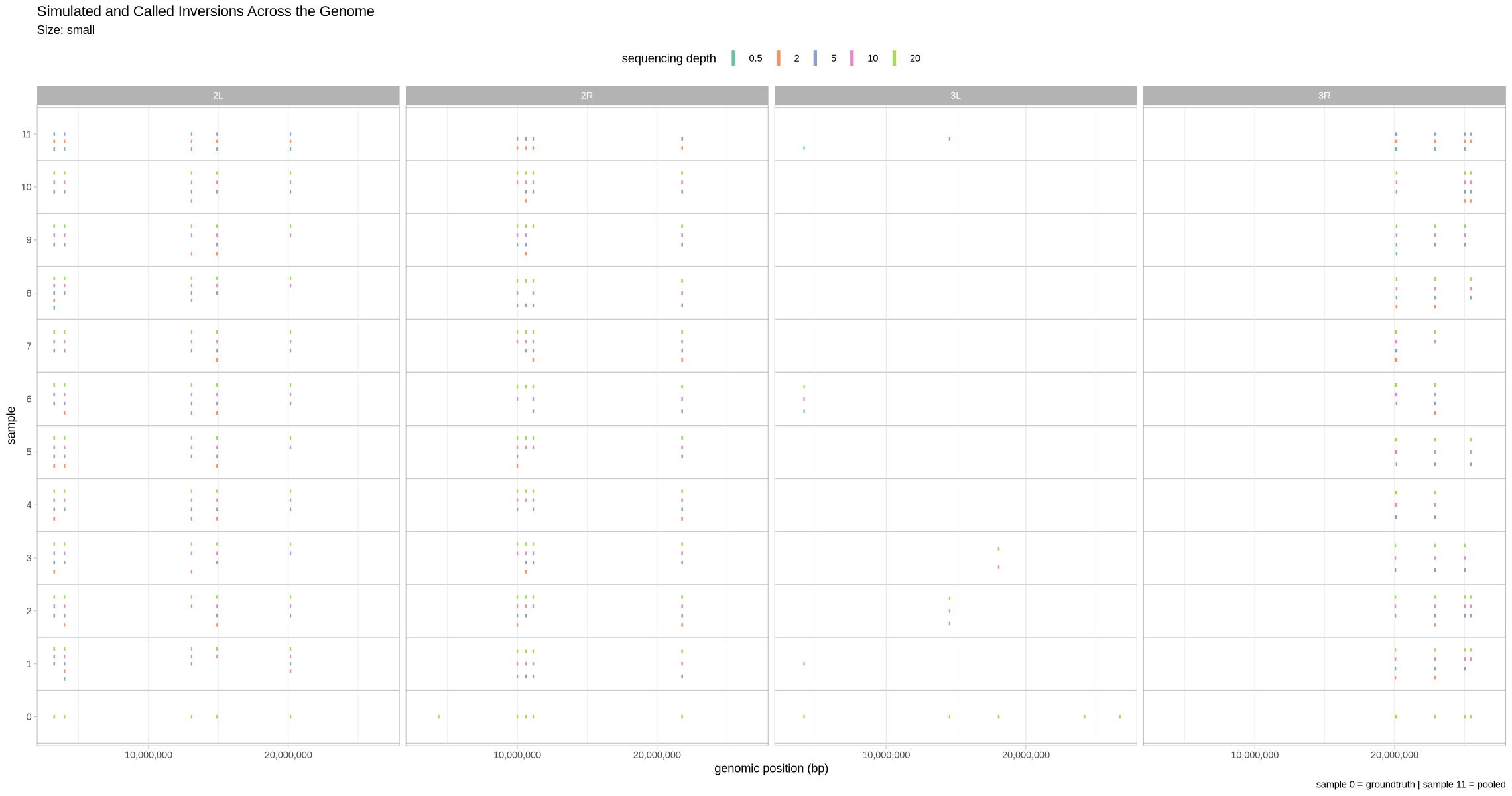
What does this look like as a heatmap of true/false positive/negative?
Source
plot_samples_scattermatrix <- function(data, size_treatment){
    options(warn = -1, repr.plot.width = 10, repr.plot.height = 15)
    .data <- data[data$sample != 11,]
    axis_ticks <- factor(paste0("sample_", sprintf("%02d", 1:10)))
    ggplot(.data, aes(y = sample, x = inversion, color = assess_cand, fill = assess_cand, shape = zygosity)) +
        geom_point(size=6) +
        theme_light() +
        labs(title = "By-Sample Inversion Detection", subtitle = paste(size_treatment, "inversions detected in individual samples, as a function of zygotic state.")) +
        scale_color_manual(name = "Assessment", values = c("false negative (undetected)" = "grey75", "false negative (filtered)" = "indianred", "true negative" = "white", "true positive" = "#90aed8")) +
        scale_fill_manual(name = "Assessment", values = c("false negative (undetected)" = "white", "false negative (filtered)" = "white", "true negative" = "white", "true positive" = "#90aed8")) +
        scale_shape_manual(name = "Zygosity", values = c("homozygous" = 21, "heterozygous" = 22)) +
        scale_x_discrete(name = "Inversion") +
        scale_y_discrete(limits = axis_ticks, breaks = axis_ticks) +
        theme(
            panel.grid.major = element_blank(),
            panel.grid.minor = element_blank()
        ) +
        facet_grid(cols = vars(contig), rows = vars(depth))
}
plot_samples_scattermatrix(performance, .size)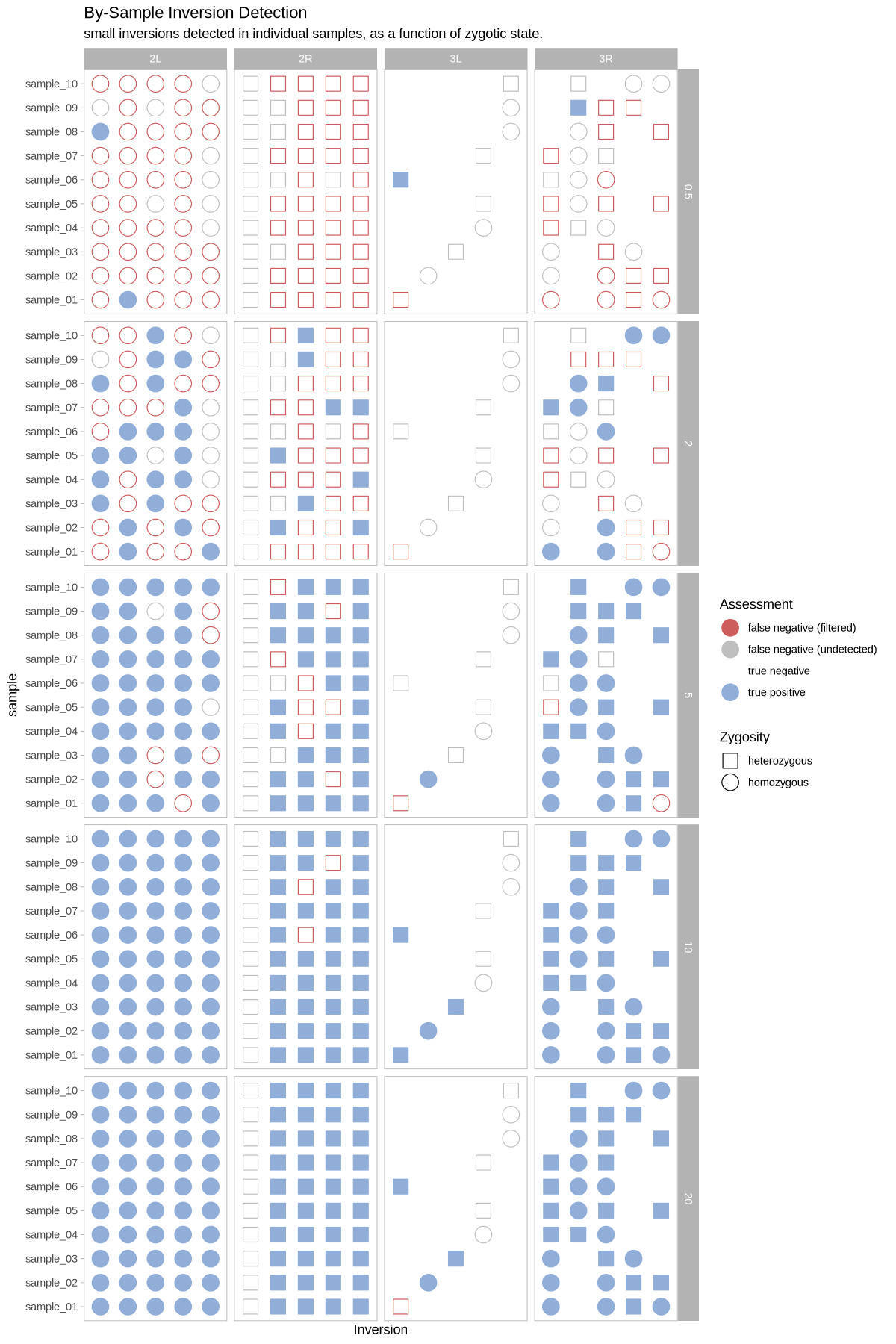
Pooled Sample Detection
Source
plot_pools_matrix <- function(data, size_treatment){
    options(warn = -1, repr.plot.width = 14, repr.plot.height = 5)
    .data <- data[data$sample == 11,]
    .data$contig <- gsub("2L", "hom", .data$contig)
    .data$contig <- gsub("2R", "het", .data$contig)
    .data$contig <- gsub("3L", "rare", .data$contig)
    .data$contig <- gsub("3R", "common", .data$contig)
    .data$contig <- factor(.data$contig,levels = c("hom","het","common", "rare"), ordered = T)

    ggplot(.data, aes(y = 1, x = inversion, color = assess_cand, fill = assess_cand)) +
        geom_point(size = 16, shape = 22) +
        theme_light() +
        labs(title = "Pooled-Sample Detection", subtitle = paste(size_treatment, "inversions detected in sample-pooled data, as a function of inversion frequency in the population.")) +
        scale_color_manual(name = "Assessment", values = c("false negative (undetected)" = "grey75", "false negative (filtered)" = "indianred", "true positive" = "#90aed8")) +
        scale_fill_manual(name = "Assessment", values = c("false negative (undetected)" = "white", "false negative (filtered)" = "white", "true negative" = "white", "true positive" = "#90aed8")) +
        scale_y_continuous(breaks = 1, name = "Assessment") +
        scale_x_discrete(name = "Inversion") +
        theme(
            panel.grid.major = element_blank(),
            panel.grid.minor = element_blank(),
            axis.text.y = element_blank(),
            axis.ticks.y = element_blank()
        ) +
        facet_grid(cols = vars(contig), rows = vars(depth))
}
plot_pools_matrix(performance, .size)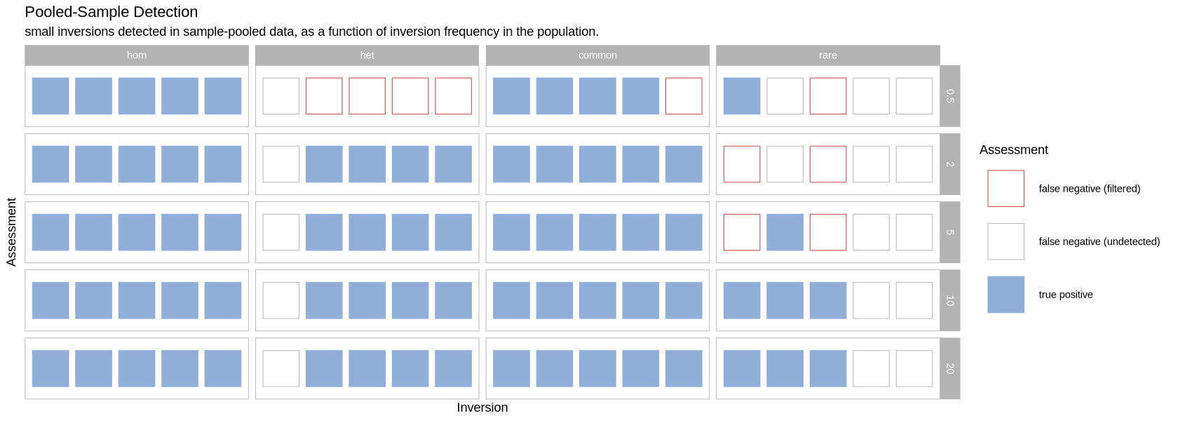
Write this all to a file to tease apart later
write.csv(performance, file = paste0(.size, ".sv.assessment"), quote = F, row.names = F)