05 Assess the Called Inversions - Inversion Simulations

Visualizing the data was useful, but we need a more rigorous solution to evaluate the results. Specifically, we are interested in the false and true positive/negative rates for each of the treatments. Lets start with loading all the variants into a tidy table. We’ll borrow the formatting code from read_data() used in the visualization steps, but it needs to be augmented to do everything and label it all.

library(dplyr)
library(tidyr)
library(ggplot2)

read_truth_data <- function(size_treatment){
    truthfile <- paste0("simulated_data/inversions/", size_treatment, "/inv.", size_treatment,".vcf")

    true_inversions <- read.table(truthfile, header = F)[,c(1,2,8)]
    true_inversions$V8 <- as.numeric(unlist(lapply(true_inversions$V8, function(X){gsub(".+END=", "", X)})))
    names(true_inversions) <- c("contig", "position_start", "position_end")
    true_inversions$size <- size_treatment
    true_inversions <- group_by(true_inversions, contig) %>%
        mutate(id = 1:n())
    return(true_inversions[, c("contig", "id","size","position_start", "position_end")])
}

read_called_data <- function(size_treatment){
    called_df <- data.frame(
        sample = character(),
        contig = character(),
        size = character(),
        depth = character(),
        position_start = numeric(),
        position_end = numeric()
    )
    for(depth in c("05X", "2X", "5X", "10X", "20X")){
        samplesfile <- paste("simulated_data/called_sv/leviathan", size_treatment, depth , "by_sample/inversions.bedpe", sep = "/")
        poolfile <- paste("simulated_data/called_sv/leviathan", size_treatment, depth, "by_pop/inversions.bedpe", sep = "/")

        sample_inversions <- read.table(
            paste("simulated_data/called_sv/leviathan", size_treatment, depth, "by_sample/inversions.bedpe", sep = "/"),
            header = T
        )[,1:4]
        if( nrow(sample_inversions) > 0){
            sample_inversions$size <- size_treatment
            sample_inversions$depth <- depth
            sample_inversions$sample <- gsub(pattern = "\\..*X", "", sample_inversions$sample)
        } else {
            sample_inversions$size <- character()
            sample_inversions$depth <- character()
        }

        pooled_inversions <- read.table(poolfile, header = T)
        pooled_inversions <- pooled_inversions[,c("population","contig", "position_start", "position_end")]
        names(pooled_inversions)[1] <- "sample"
        if( nrow(pooled_inversions) > 0){
            pooled_inversions$sample <- "pooled"
            pooled_inversions$size <- size_treatment
            pooled_inversions$depth <- depth
        } else {
            pooled_inversions$size <- character()
            pooled_inversions$depth <- character()
        }
        called_df <- rbind(called_df, sample_inversions, pooled_inversions)
    }

    return(called_df)
}

Read in data¶

The assessment process is a little tricky, so let’s start by having one dataframe of the known inversions and another of the called inversions. Using Reduce(rbind, Map()) is going to make life a lot easier here.

Known inversions¶

truthset <- Reduce(rbind, Map(read_truth_data, c("small","medium","large","xl")))
head(truthset)
tail(truthset)

Called inversions¶

These are the inversions that LEVIATHAN called.

calledset <- Reduce(rbind, Map(read_called_data, c("small","medium","large","xl")))
head(calledset)
tail(calledset)

Known sample inversions¶

I think it might make sense to do a fuzzy-match for the inversions for a given size treatment. Fuzzy in the sense that the start/end positions of the called inversions can be something like 1kb away and from the known breakpoint and still count.

Considerations:

we are interested in the True/False Negative/Positive at all treatment levels
not every sample has every simulated inversion.
- we need to get the table of which samples have which inversions and cross-reference that to make sure that the presence/absence is actually true

inv_inventory <- read.table("inversion_simulations.inventory", header = T)
names(inv_inventory)[4] <- "id"
head(inv_inventory)

We also need to add the pooled samples to this inventory

pool_inventory <- read.table("inversion_simulations.pool.inventory", header = T)
names(pool_inventory)[4] <- "id"
inv_inventory <- rbind(inv_inventory, pool_inventory)
tail(inv_inventory)

We need to combine the inventory of samples’ inversions (inv_inventory) it with the known inversions themselves (truthset) to get an adequate table to iterate through. Doing a left join will give us that.

inv_inventory <- left_join(inv_inventory, truthset, by = c("contig","id", "size"))
head(inv_inventory)

Match called and known inversions¶

Next comes what should be a big loop that goes through rows of inv_inventory (an inversion for a sample) and checks calledset for if that inversion was called. We will need a nested loop that (outer loop) iterates through the depth treatments and an inner loop that iterates through the big inventory manifest (inv_inventory).

So now we loop through inv_inventory and try to match calls in calledset, adjusting the count column as necessary (booleans are easy to sum)

check the callset for that inversion on that contig in that sample at that depth
- if inv_inventory$present is TRUE, then and it is there, it’s a TRUE POSITIVE
- if inv_inventory$present is TRUE, then and it’s not there, it’s a FALSE NEGATIVE
- if inv_inventory$present is FALSE, then and it is there, it’s a FALSE POSITIVE
- if inv_inventory$present is FALSE, then and it’s not there, it’s a TRUE NEGATIVE

all while doing a fuzzy match of 1 kbp

The is_called() function below will do all that. It takes a row from inv_inventory as input and will try to fuzzy-match the known inversion in the set of called inversions (calledset). One row goes in, but four rows get outputted (one row each for True/False Positive/Negative), and the resulting 4-row dataframe will be appended onto a growing results dataframe assessment. This 1-to-4 conversion makes the resulting dataframe in long-format, which will make math and plotting easier.

is_called <- function(query_row, called_sv, depth_treatment, fuzzy_distance){
    # the vector returned corresponds to c(TP, FP, TN, FN)
    samplename <- query_row$sample
    sizeclass <- query_row$size
    # add padding to make the breakpoints more generous
    fuzzy_start <- query_row$position_start - fuzzy_distance
    fuzzy_end <- query_row$position_end + fuzzy_distance
    q_contig <- query_row$contig
    present <- query_row$present
    filtered_called <- filter(
        called_sv,
        sample == samplename,
        contig == q_contig,
        size == sizeclass,
        depth == depth_treatment,
        position_start >= fuzzy_start,
        position_end <= fuzzy_end
    )
    hits <- nrow(filtered_called)
    check_vec <- c(FALSE, FALSE, FALSE, FALSE)
    if(present){
        if(hits > 0){
            check_vec[1] <- TRUE
        } else {
            check_vec[4] <- TRUE
        }
    } else {
        if(hits > 0){
            check_vec[2] <- TRUE
        } else {
            check_vec[3] <- TRUE
        }
    }
    out_rows <- query_row[rep(1,4), ]
    out_rows$depth <- depth_treatment
    out_rows$assessment <- c("True Positive", "False Positive", "True Negative", "False Negative")
    out_rows$count <- check_vec
    return(out_rows)
}

depths <- c("05X", "2X", "5X", "10X", "20X")
assessment <- data.frame(
    sample = character(),
    size = character(),
    contig = character(),
    id = integer(),
    present = logical(),
    state = character(),
    position_start = integer(),
    position_end = integer(),
    depth = character(),
    assessment = character(),
    count = logical()
)
for(.depth in depths){
    for(i in 1:nrow(inv_inventory)){
        results <- is_called(inv_inventory[i,], calledset, .depth , 1000)
        assessment <- rbind(assessment, results)
    }
}
assessment$depth <- factor(assessment$depth, levels = depths)
assessment$size <- factor(assessment$size, levels = c("small", "medium", "large", "xl"))
# fix pooled-sample state to hom to avoid NA
assessment$state[is.na(assessment$state)] <- "hom"
head(assessment)

Summarize by size-contig-depth¶

Given that the contigs themselves are also treatments, it might be useful to aggregate within the contigs for a depth treatment. We’ll include an absolute count and a percent ratio, as that might be more informative.

assessment_by_contig <- group_by(assessment, size, contig, depth, assessment) %>%
    summarize_at("count", ~ sum(.x)) %>%
    group_by(size, contig, depth) %>%
    mutate(percent = round(count/sum(count) * 100,2))
head(assessment_by_contig)

ggplot(assessment_by_contig, aes(x = depth, y = count, color = assessment, group = assessment)) +
    geom_point() +
    geom_line() +
    theme_light() +
    facet_grid(rows = vars(contig), cols = vars(size), scales = "free_y")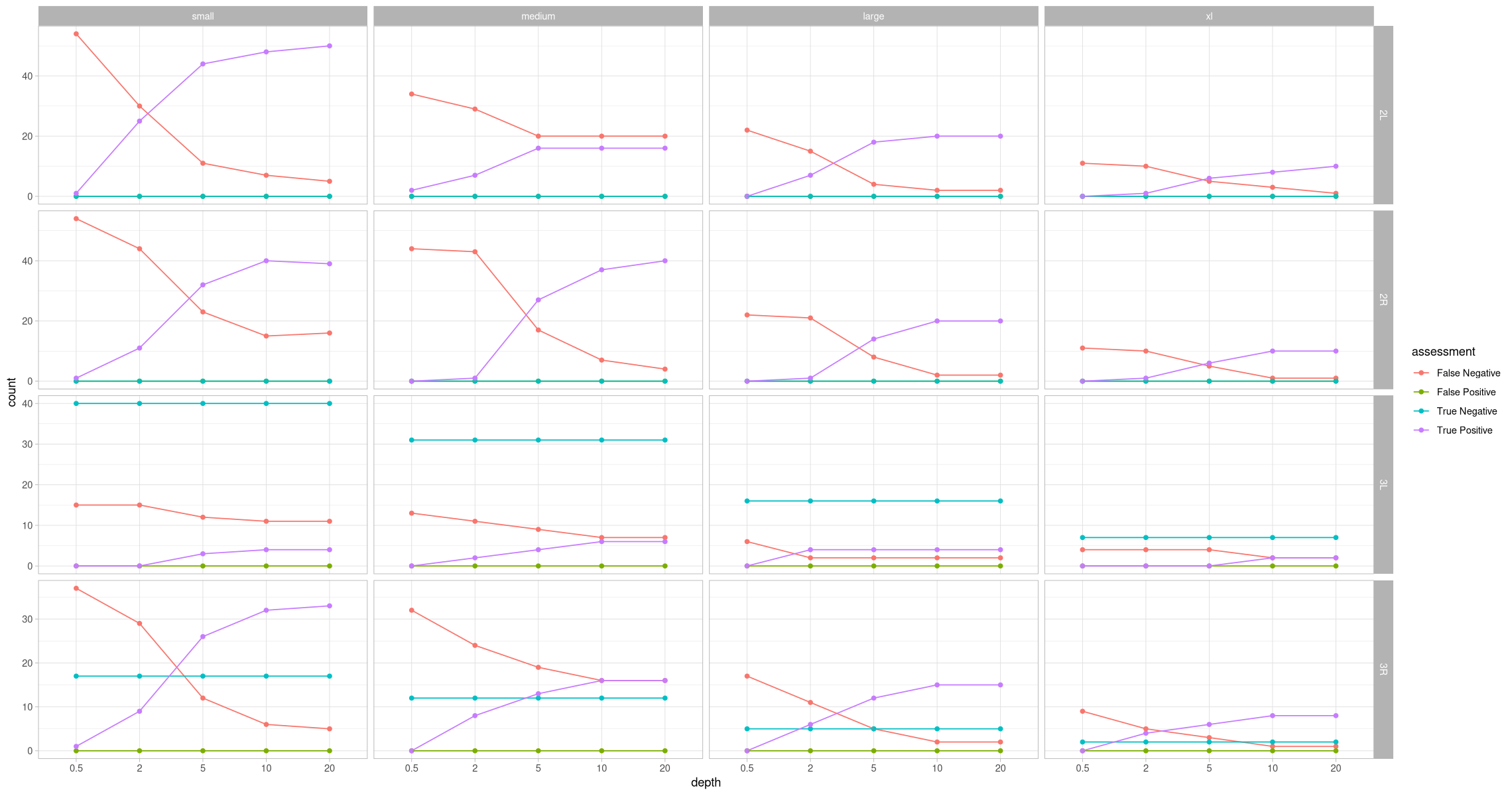

Let’s plot it with percentages, which should be more revealing

ggplot(assessment_by_contig, aes(x = depth, y = percent, color = assessment, group = assessment)) +
    geom_point() +
    geom_line() +
    theme_light() +
    facet_grid(rows = vars(contig), cols = vars(size))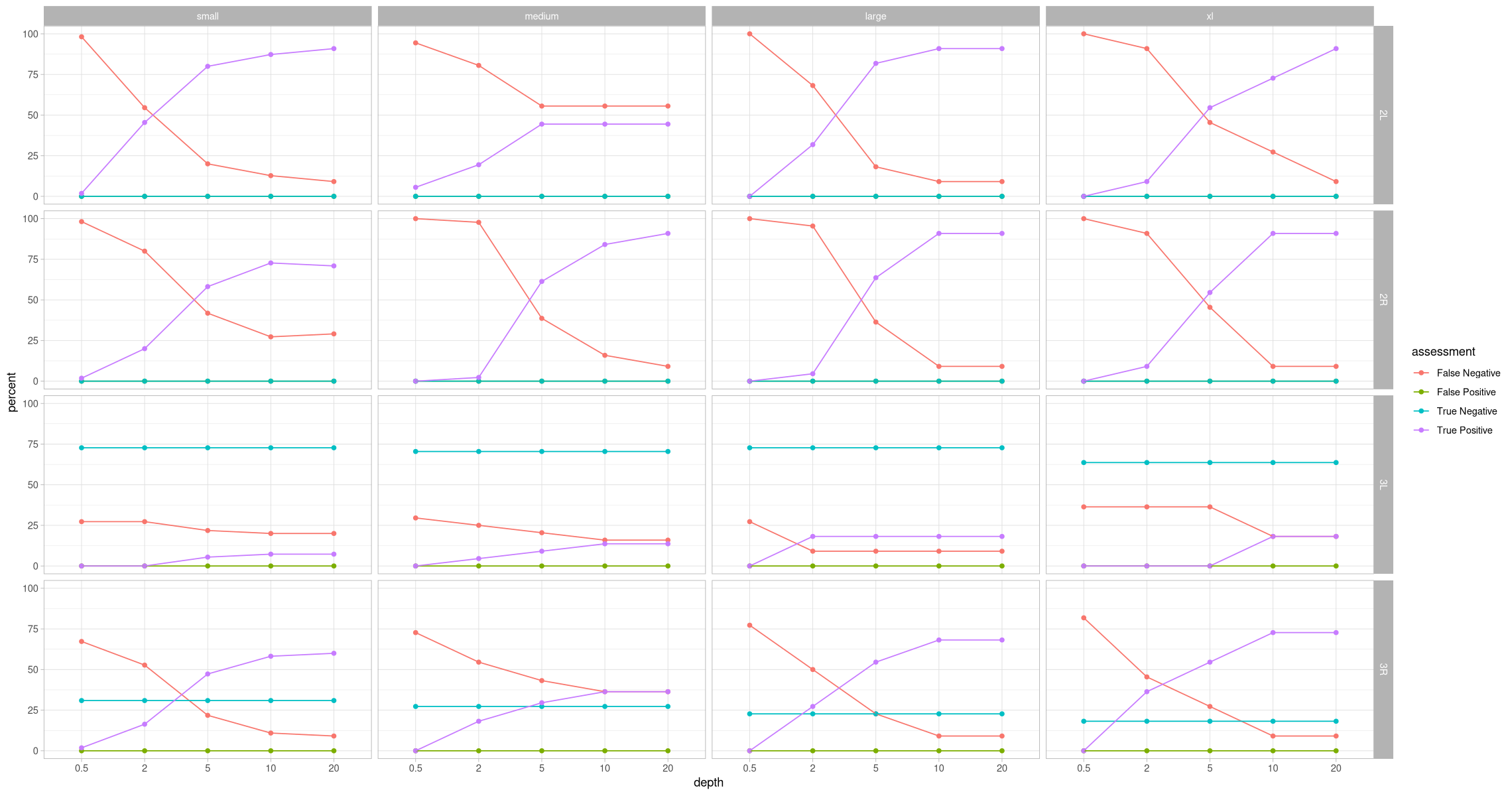

Summarize by zygosity¶

Oh hey, that’s looking like something. Pretty exciting, actually. There are no false positives, which is great. What about what this looks like taking the zygosity into consideration? Let’s also add a percent in addition to the absolute count.

assessment_by_contig_state <- group_by(assessment, size, state, contig, depth, assessment) %>% 
    summarize_at("count", ~ sum(.x)) %>%
    group_by(size, state, contig, depth) %>%
    mutate(percent = count/sum(count) * 100)
head(assessment_by_contig_state)

ggplot(assessment_by_contig_state, aes(x = depth, y = count, color = assessment, shape = state, group = paste(assessment, state))) +
    geom_point() +
    geom_line(aes(linetype = state)) +
    theme_light() +
    facet_grid(rows = vars(contig), cols = vars(size), scales = "free_y")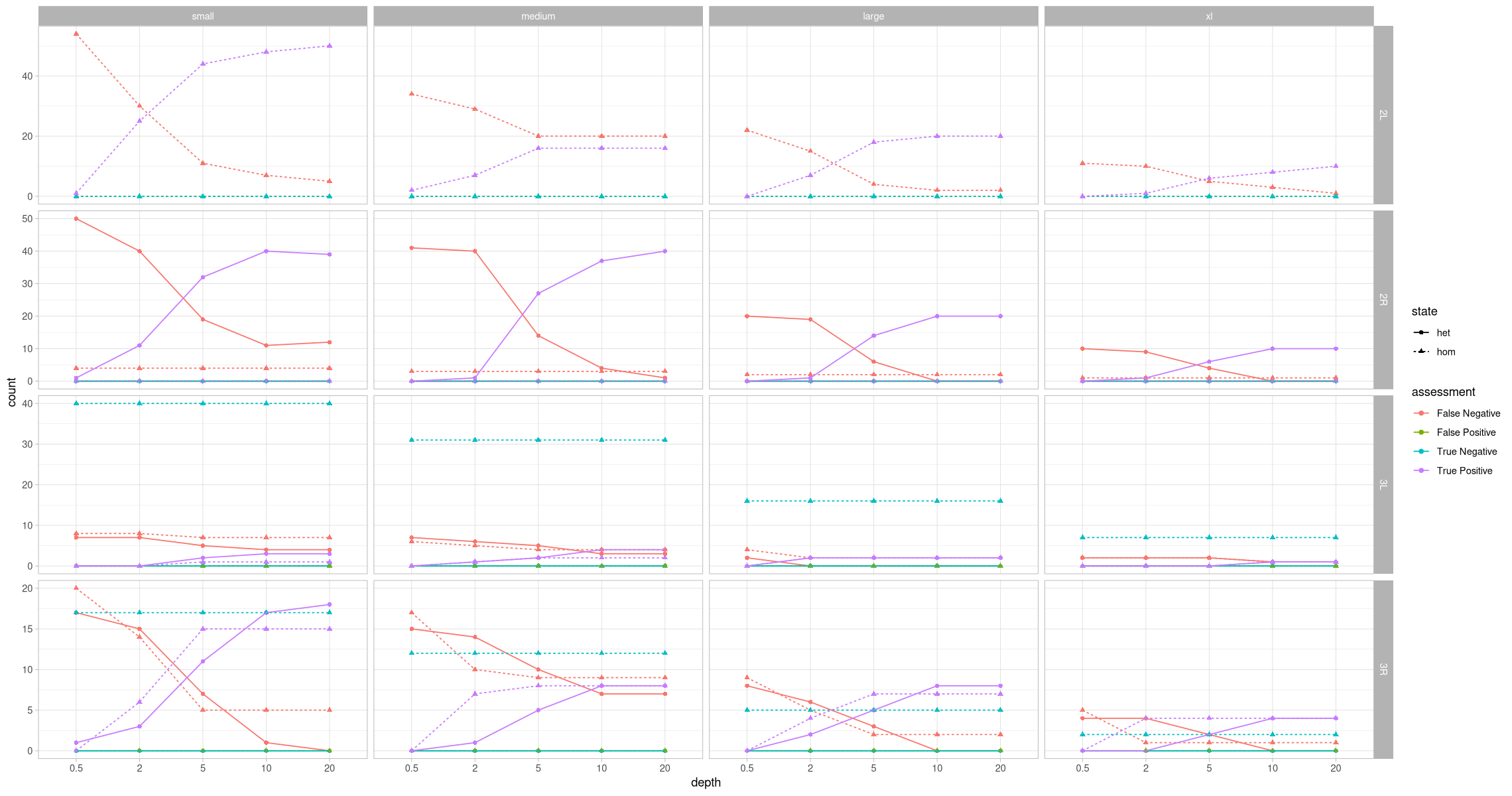

Let’s plot it with ratios again

ggplot(assessment_by_contig_state, aes(x = depth, y = percent, color = assessment, shape = state, group = paste(assessment, state))) +
    geom_point() +
    geom_line(aes(linetype = state)) +
    theme_light() +
    facet_grid(rows = vars(contig), cols = vars(size))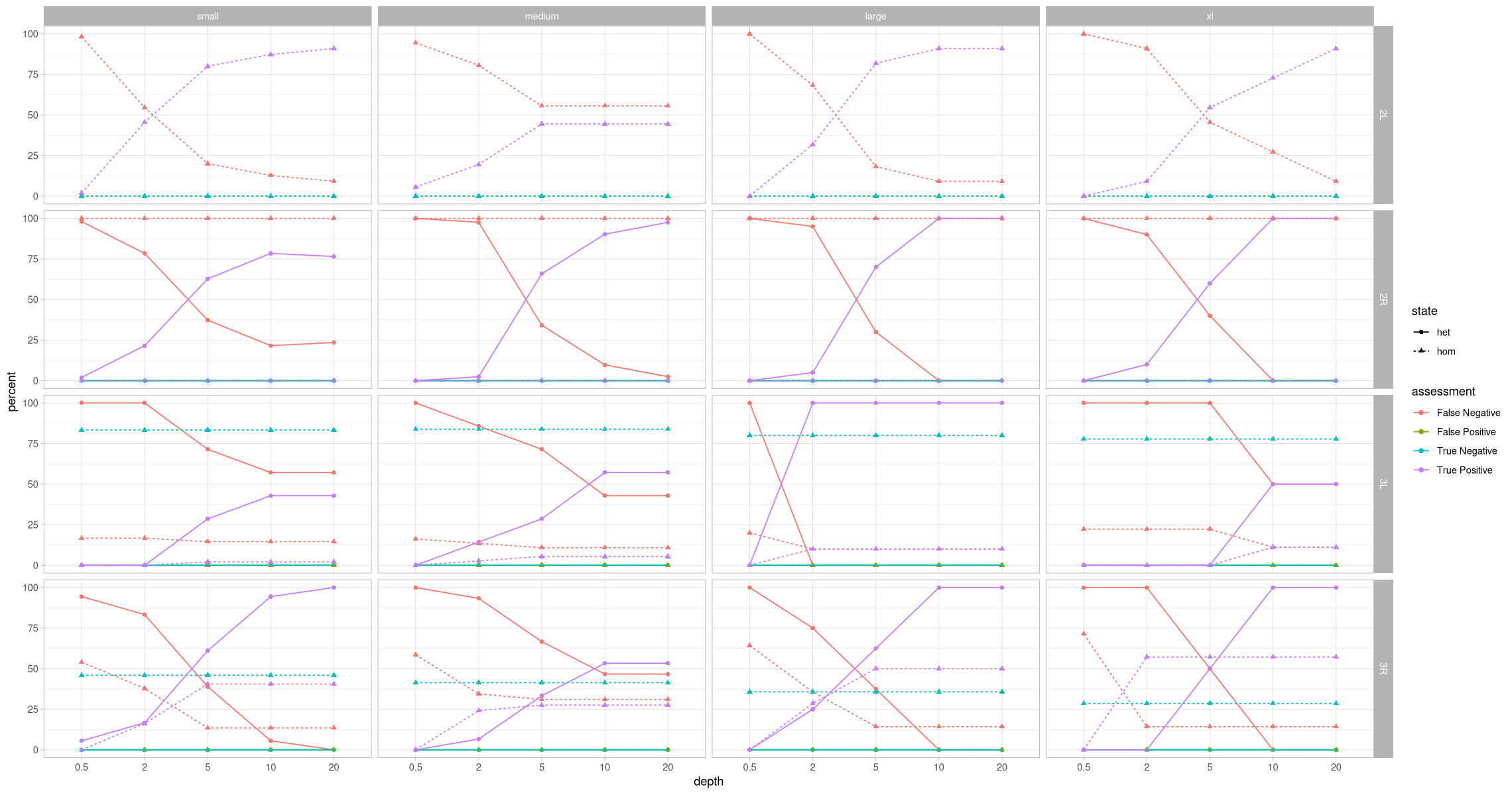

Splitting the positives and negatives¶

These plots don’t communicate the situation necessarily accurately because there can be 75% true negatives of all possible states, but the true negative identification rate is actually 100%. So, let’s split the data into samples that have an inversion simulated onto them and ones that done, then plot the positives separately from the negatives.

Inversion was present¶

assessment_positive_contig <- filter(assessment, present, assessment %in% c("True Positive", "False Negative")) %>% group_by(size, contig, depth, assessment) %>% 
    summarize_at("count", ~ sum(.x)) %>%
    group_by(size, contig, depth) %>%
    mutate(percent = count/sum(count) * 100)
head(assessment_positive_contig)

ggplot(assessment_positive_contig, aes(x = depth, y = percent, color = assessment, group = assessment)) +
    geom_point() +
    geom_line() +
    theme_light() +
    facet_grid(rows = vars(contig), cols = vars(size))

Inversion was absent¶

assessment_negative_contig <- filter(assessment, !present, assessment %in% c("True Negative", "False Positive")) %>% group_by(size, contig, depth, assessment) %>% 
    summarize_at("count", ~ sum(.x)) %>%
    group_by(size, contig, depth, assessment) %>%
    mutate(percent = count/sum(count) * 100)

assessment_negative_contig$percent[is.na(assessment_negative_contig$percent)] <- 0
head(assessment_negative_contig)

ggplot(assessment_negative_contig, aes(x = depth, y = percent, color = assessment, group = assessment)) +
    geom_point() +
    geom_line() +
    theme_light() +
    facet_grid(rows = vars(contig), cols = vars(size))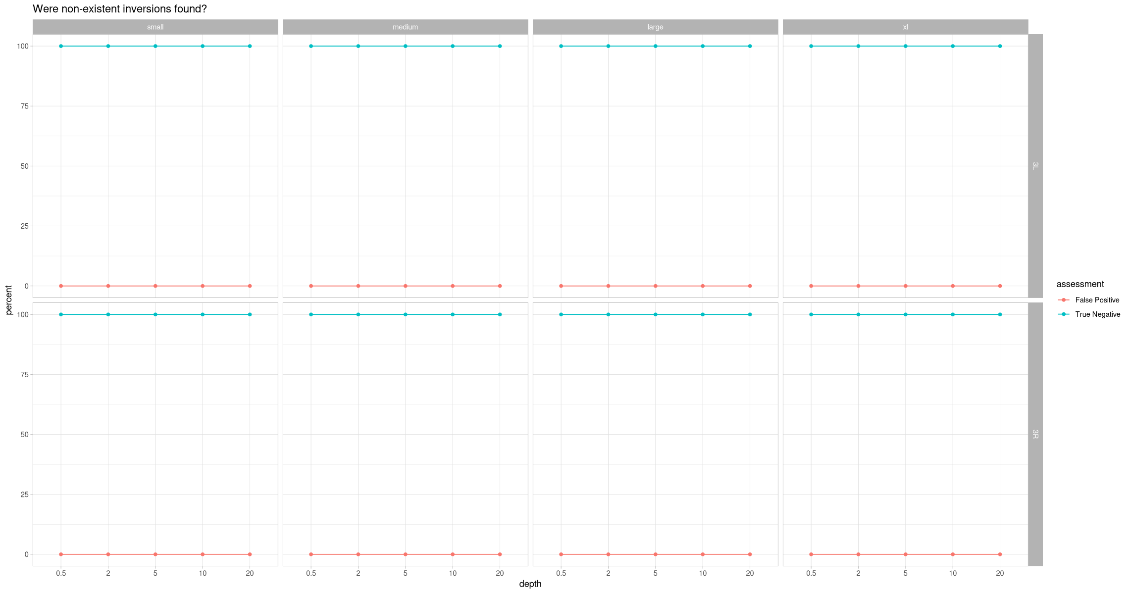

Inversion was present (zygosity)¶

assessment_positive_contig_state <- filter(assessment, present, assessment %in% c("True Positive", "False Negative")) %>% group_by(size, state, contig, depth, assessment) %>% 
    summarize_at("count", ~ sum(.x)) %>%
    group_by(size, state, contig, depth) %>%
    mutate(percent = count/sum(count) * 100)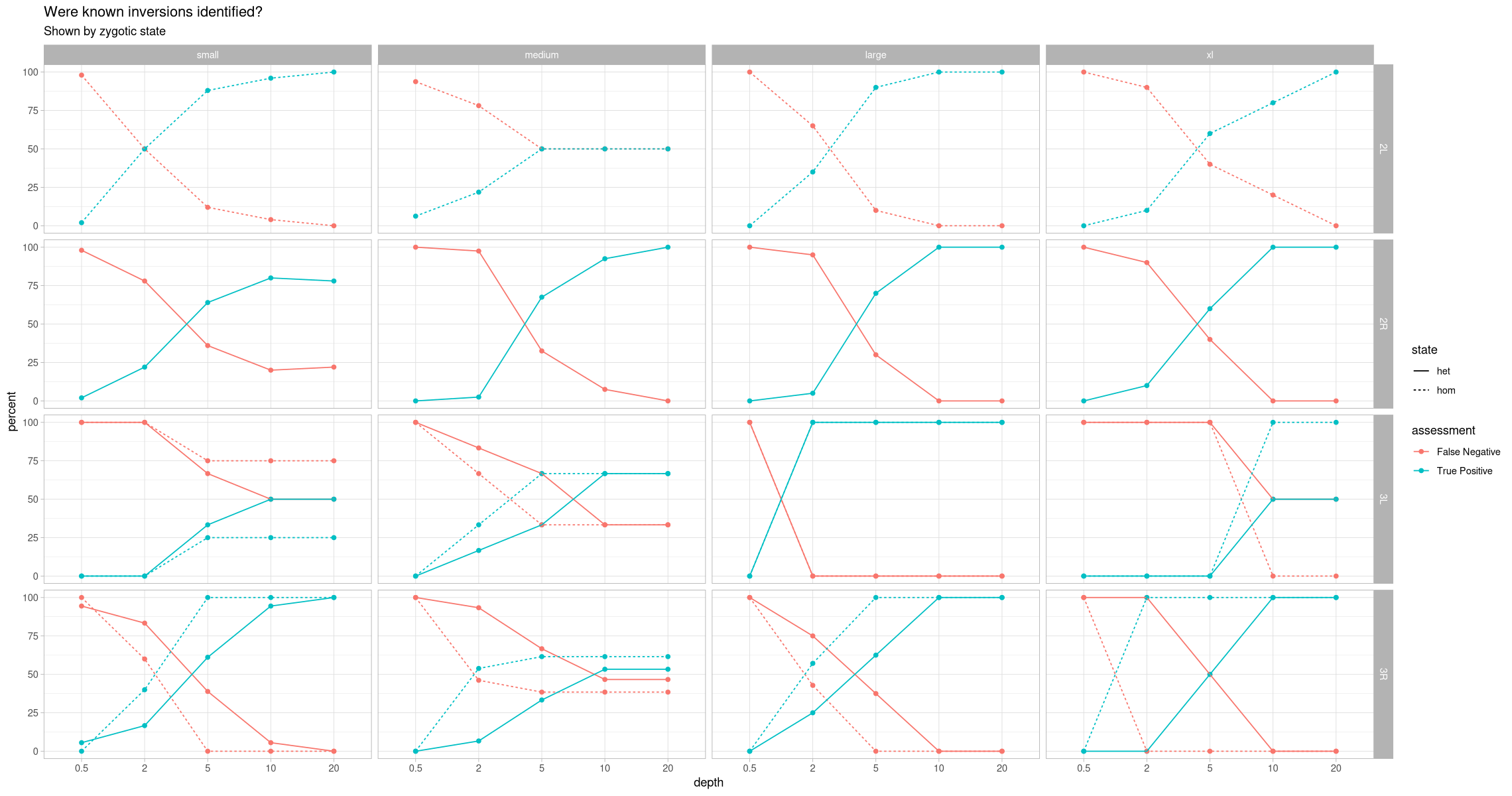
head(assessment_positive_contig_state)

ggplot(assessment_positive_contig_state, aes(x = depth, y = percent, color = assessment, group = paste(assessment, state))) +
    geom_point() +
    geom_line(aes(linetype = state)) +
    theme_light() +
    facet_grid(rows = vars(contig), cols = vars(size))

Inversion was absent (zygosity)¶

assessment_negative_contig_state <- filter(assessment, !present, assessment %in% c("True Negative", "False Positive")) %>% group_by(size, state, contig, depth, assessment) %>% 
    summarize_at("count", ~ sum(.x)) %>%
    group_by(size, state, contig, depth, assessment) %>%
    mutate(percent = count/sum(count) * 100)

assessment_negative_contig_state$percent[is.na(assessment_negative_contig_state$percent)] <- 0
head(assessment_negative_contig_state)

ggplot(assessment_negative_contig_state, aes(x = depth, y = percent, color = assessment, group = paste(assessment, state))) +
    geom_point() +
    geom_line(aes(linetype = state)) +
    theme_light() +
    facet_grid(rows = vars(contig), cols = vars(size))

Inversion Simulations

XL-sized Inversions