Linked-Read (NAIBR) - Inversion Simulations

Here, we aggregate the visualizations of all size classes and depth treatments for linked-read simulations.

library(dplyr)
library(ggplot2)
library(ggpubr)
library(tidyr)


Attaching package: 'dplyr'


The following objects are masked from 'package:stats':

    filter, lag


The following objects are masked from 'package:base':

    intersect, setdiff, setequal, union

Let’s read in the data from the outcomes of the individual size-class assessments and combine them into a single table. Since we’ll be comparing this to the long-read data, we should also add a column specifing this is linked-read data and write the entire thing into one file.

lr_inversions <- rbind(
    read.csv("small.sv.naibr.assessment", header = T),
    read.csv("medium.sv.naibr.assessment", header = T),
    read.csv("large.sv.naibr.assessment", header = T),
    read.csv("xl.sv.naibr.assessment", header = T)
)
lr_inversions$technology <- "linkedread"
lr_inversions$method <- "naibr"
if(!file.exists("linkedread.sv.assessment")){
    write.csv(lr_inversions, file = "linkedread.sv.assessment", row.names = F, quote = F)
}
head(lr_inversions)

false_positives <- Reduce(
    rbind,
    Map(
        function(x){ read.table(x, header = T)},
        list.files(pattern = "false_positives*",full.names = T)
    )
)
false_positives$assessment <- "false positive"
head(false_positives)

Summary statistics¶

We need to know things like:

Per Sample-Size-Depth

average number of identified inversions
average number of false positives
recall
precision
$F_{1}$ score

The assessment and FP table aren’t in the same format, so it would be easier to trim down the bigger table and append the false positive one to it, then do the summary stats.

.inversions <- select(lr_inversions, contig, position_start, position_end, sample, depth, size, assessment, method)
.inversions$datatype <- ifelse(.inversions$sample == 11, "pooled", "single-sample")
head(.inversions)

It may be worth collapsing these into averages across size-depth treatments (averaging across samples)

metrics <- group_by(.inversions, size, depth, datatype) %>%
    summarize(
        TP = sum(assessment == "true positive"),
        FP = sum(assessment == "false positive"),
        TN = sum(assessment == "true negative"),
        FN = sum(assessment == "false negative")
    ) %>% ungroup()
metrics$precision <- metrics$TP / (metrics$TP + metrics$FP)
metrics$recall <- metrics$TP / (metrics$TP + metrics$FN)
metrics$F1 <- 2 * ((metrics$precision * metrics$recall) / (metrics$precision + metrics$recall))
metrics$depth <- metrics$depth
metrics$size <- factor(metrics$size, ordered = T, levels = c("small", "medium", "large", "xl"))
head(metrics)

`summarise()` has grouped output by 'size', 'depth'. You can override using the
`.groups` argument.

greys <- c(
    "#c0c6cf",
    "#a2aab5",
    "#6e7684",
    "#54546c",
    "black"
)

colorful <- c(
    "#9b6981",
    "#682c37",
    "#f6955e" ,
    "#a8cdec"
)

options(warn = -1, repr.plot.width = 10, repr.plot.height = 10)
ggplot(metrics, aes(x = depth, y = F1, color = size, shape = datatype, group = paste(size, datatype), linetype = datatype)) +
    geom_line() +
    geom_point(size = 6) +
    theme_light() +
    scale_shape_manual(name = "Data Type", values = c(19, 15)) +
    scale_color_manual(name = "Inversion Size", values = colorful) +
    scale_linetype_manual(name = "Data Type", values = c("pooled" = "dashed", "single-sample" = "solid")) +
    labs(title = "F-scores Across treatments (NAIBR)")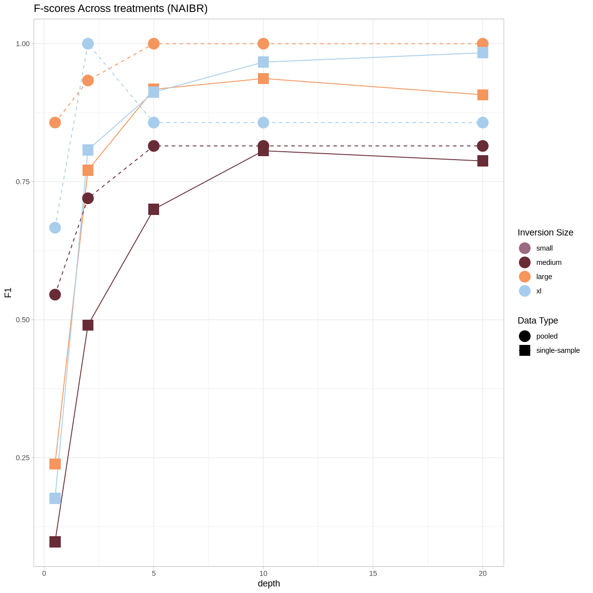

options(warn = -1, repr.plot.width = 15, repr.plot.height = 7.5)
ggplot(metrics, aes(x = recall, y = precision, color = as.factor(depth), shape = size)) +
    geom_point(size = 6) +
    geom_abline(intercept = 0, slope = 1) +
    theme_light() +
    scale_color_manual(name = "Single-Sample Depth", values = greys) +
    scale_shape_manual(name = "Inversion Size", values = c(19,15,18,17)) +
    coord_cartesian(xlim = c(0,1), ylim = c(0,1)) +
    labs(title = "Precision-Recall Curve (NAIBR)") +
    facet_grid(cols = vars(datatype))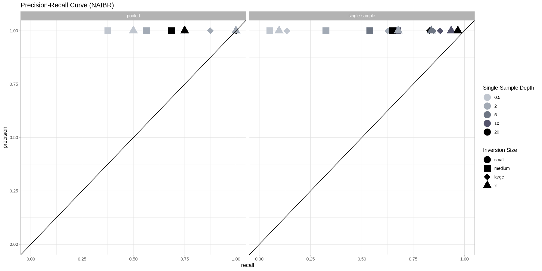

Single-Sample Detection¶

Let’s visualize what detection looked like across all treatments with respect to false/true positive/negative. Here, we facet rows across depths and show all the size treatments across columns.

options(warn = -1, repr.plot.width = 20, repr.plot.height = 15)
axis_ticks <- factor(paste0("sample_", sprintf("%02d", 1:10)))
lr_inversions[lr_inversions$sample != 11,] %>%
    ggplot(aes(y = sample, x = id, color = assessment, fill = assessment, shape = zygosity)) +
        geom_point(size=6) +
        theme_light() +
        labs(title = "By-Sample Inversion Detection (NAIBR)", subtitle = "Inversions detected in individual samples, as a function of zygotic state.") +
        scale_color_manual(name = "Assessment", values = c("false negative" = "grey75", "true negative" = "white", "true positive" = "#90aed8")) +
        scale_fill_manual(name = "Assessment", values = c("false negative" = "white", "true negative" = "white", "true positive" = "#90aed8")) +
        scale_shape_manual(values = c("homozygous" = 21, "heterozygous" = 22)) +
        scale_x_discrete(name = "Inversion") +
        scale_y_discrete(limits = axis_ticks, breaks = axis_ticks) +
        theme(
            panel.grid.major = element_blank(),
            panel.grid.minor = element_blank()
        ) +
        facet_grid(depth ~ factor(size, levels = c("small", "medium", "large", "xl")), scales = "free_x")

Pooled Sample Detection¶

plot_pools_matrix <- function(data, size_treatment){
    .data <- data[data$sample == 11 & data$size == size_treatment,]
    .data$contig <- gsub("2L", "hom", .data$contig)
    .data$contig <- gsub("2R", "het", .data$contig)
    .data$contig <- gsub("3L", "rare", .data$contig)
    .data$contig <- gsub("3R", "common", .data$contig)
    .data$contig <- factor(.data$contig,levels = c("hom","het","common", "rare"), ordered = T)

    ggplot(.data, aes(y = 1, x = inversion, color = assessment, fill = assessment)) +
        geom_point(size=8, shape = 22) +
        theme_light() +
        scale_color_manual(name = "Assessment", values = c("false negative" = "grey75", "true positive" = "#90aed8")) +
        scale_fill_manual(name = "Assessment", values = c("false negative" = "white", "true negative" = "white", "true positive" = "#90aed8")) +
        scale_y_continuous(breaks = 1, name = "") +
        scale_x_discrete(name = "Inversion") +
        theme(
            panel.grid.major = element_blank(),
            panel.grid.minor = element_blank(),
            axis.text.y = element_blank(),
            axis.ticks.y = element_blank(),
            axis.label.y = element_blank()
        ) +
        facet_grid(cols = vars(contig), rows = vars(depth))
}

options(warn = -1, repr.plot.width = 20, repr.plot.height = 3.5)
plot <- ggarrange(
    plot_pools_matrix(lr_inversions, "small"),
    plot_pools_matrix(lr_inversions, "medium"),
    plot_pools_matrix(lr_inversions, "large"),
    plot_pools_matrix(lr_inversions, "xl"),
    labels = c("small", "medium", "large", "xl"),
    nrow = 1, ncol = 4, common.legend = T, font.label = c(face = "plain"), legend = "top",
    vjust = 0, label.x = c(0.43, 0.38, 0.38, 0.47),
    widths = c(1, .75, .50, .40)
)
annotate_figure(
    plot,
    top = text_grob(
        "Pooled-Sample Detection (NAIBR)", color = "black", size = 20
        )
)